Complex branches: turns, loops, retrograde motion, and mixed futures

This tutorial shows how to interpret biologically unusual velocity fields without forcing every annotated branch into a monotonic outward ray.

The core distinction is:

• Conditional Fate Affinity (CFA) describes future identity;

• Discounted Fate Reach (DFR) describes how much selected-fate probability is resolved;

• Future-Fate Specificity (FFS) describes decisiveness;

• Signed Ordering Flux (SOF) describes forward or retrograde movement.

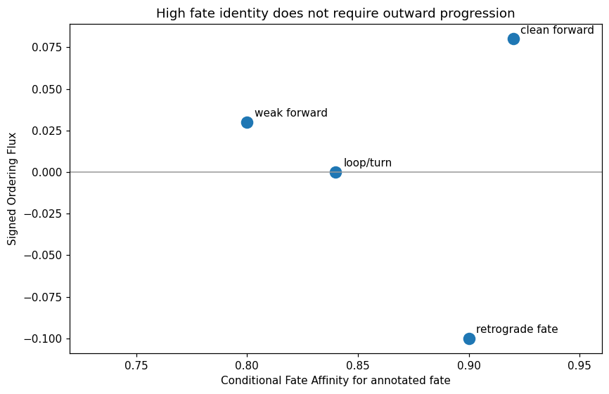
A branch can have high CFA for its annotated fate and negative or sign-changing SOF. That is not a contradiction.

1. Imports and synthetic archetypes

from __future__ import annotations

import matplotlib.pyplot as plt
import numpy as np
import pandas as pd

import scCS

SEED = 20260714
rng = np.random.default_rng(SEED)
plt.rcParams["figure.dpi"] = 110

print("scCS", scCS.__version__)

scCS 0.8.0.dev34

2. Formal separation of identity and motion

DFFP fate identity is based on the conditional probability vector \(q_i\). Signed Ordering Flux uses the supplied ordering \(s\):

\[\widetilde P_{ij}=\frac{P_{ij}}{\sum_{k\in S}P_{ik}},\qquad g_i=\sum_{j\in S}\widetilde P_{ij}(s_j-s_i).\]

There is no equation requiring high \(q_{if}\) to imply positive \(g_i\). A cell may retain high affinity for fate \(f\) while returning toward an earlier state, following a loop, or turning across the embedding.

identity_motion = pd.DataFrame(
    {
        "CFA for annotated fate": [0.92, 0.90, 0.84, 0.80],
        "SOF": [0.08, -0.10, 0.00, 0.03],
        "case": ["clean forward", "retrograde fate", "loop/turn", "weak forward"],
    }
)
fig, ax = plt.subplots(figsize=(8, 5.2))
ax.scatter(identity_motion["CFA for annotated fate"], identity_motion["SOF"], s=110)
for _, row in identity_motion.iterrows():
    ax.annotate(
        row["case"],
        (row["CFA for annotated fate"], row["SOF"]),
        xytext=(7, 5),
        textcoords="offset points",
    )
ax.axhline(0, color="0.6", linewidth=1)
ax.set_xlim(0.72, 0.96)
ax.set_xlabel("Conditional Fate Affinity for annotated fate")
ax.set_ylabel("Signed Ordering Flux")
ax.set_title("High fate identity does not require outward progression")
fig.tight_layout()
plt.show()

3. Branch-relative display angles

For a display velocity \(v_i\), decompose it into components parallel and perpendicular to the annotated branch direction \(d_f\):

\[v_{\parallel}=v_i^\top d_f,\qquad v_{\perp}=v_i-v_{\parallel}d_f,\qquad \theta_i=\operatorname{atan2}(\|v_{\perp}\|,v_{\parallel}).\]

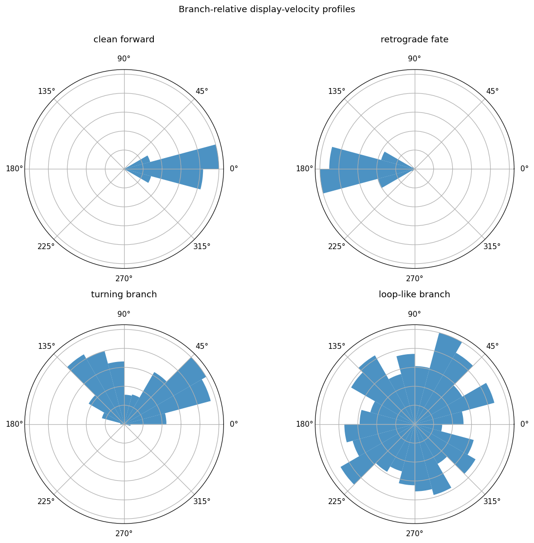
Thus \(0^\circ\) is outward, \(180^\circ\) is inward, and \(\pm90^\circ\) is transverse. These angles are display diagnostics only; DFFP remains defined on the source graph.

t = np.linspace(0.0, 1.0, 120)

archetypes = {
    "clean forward": {
        "x": t,
        "y": np.zeros_like(t),
        "flux": 0.08 + 0.02 * np.sin(np.pi * t),
        "affinity": 0.90 + 0.05 * t,
        "reach": 0.55 + 0.35 * t,
    },
    "retrograde fate": {
        "x": t,
        "y": 0.05 * np.sin(np.pi * t),
        "flux": -0.04 - 0.10 * t,
        "affinity": 0.82 + 0.10 * t,
        "reach": 0.45 + 0.30 * t,
    },
    "turning branch": {
        "x": t,
        "y": 0.45 * np.sin(np.pi * t),
        "flux": 0.11 * np.cos(np.pi * t),
        "affinity": 0.78 + 0.08 * np.sin(np.pi * t),
        "reach": 0.40 + 0.40 * t,
    },
    "loop-like branch": {
        "x": 0.55 + 0.38 * np.cos(2 * np.pi * t),
        "y": 0.38 * np.sin(2 * np.pi * t),
        "flux": 0.13 * np.cos(2 * np.pi * t),
        "affinity": 0.74 + 0.12 * np.cos(np.pi * (t - 0.5)),
        "reach": 0.35 + 0.35 * t,
    },
}
for values in archetypes.values():
    values["specificity"] = np.clip(
        0.15 + 0.85 * (values["affinity"] - 0.25) / 0.75,
        0,
        1,
    )
    values["resolved"] = values["reach"] * values["specificity"]

4. Source-space velocity archetypes

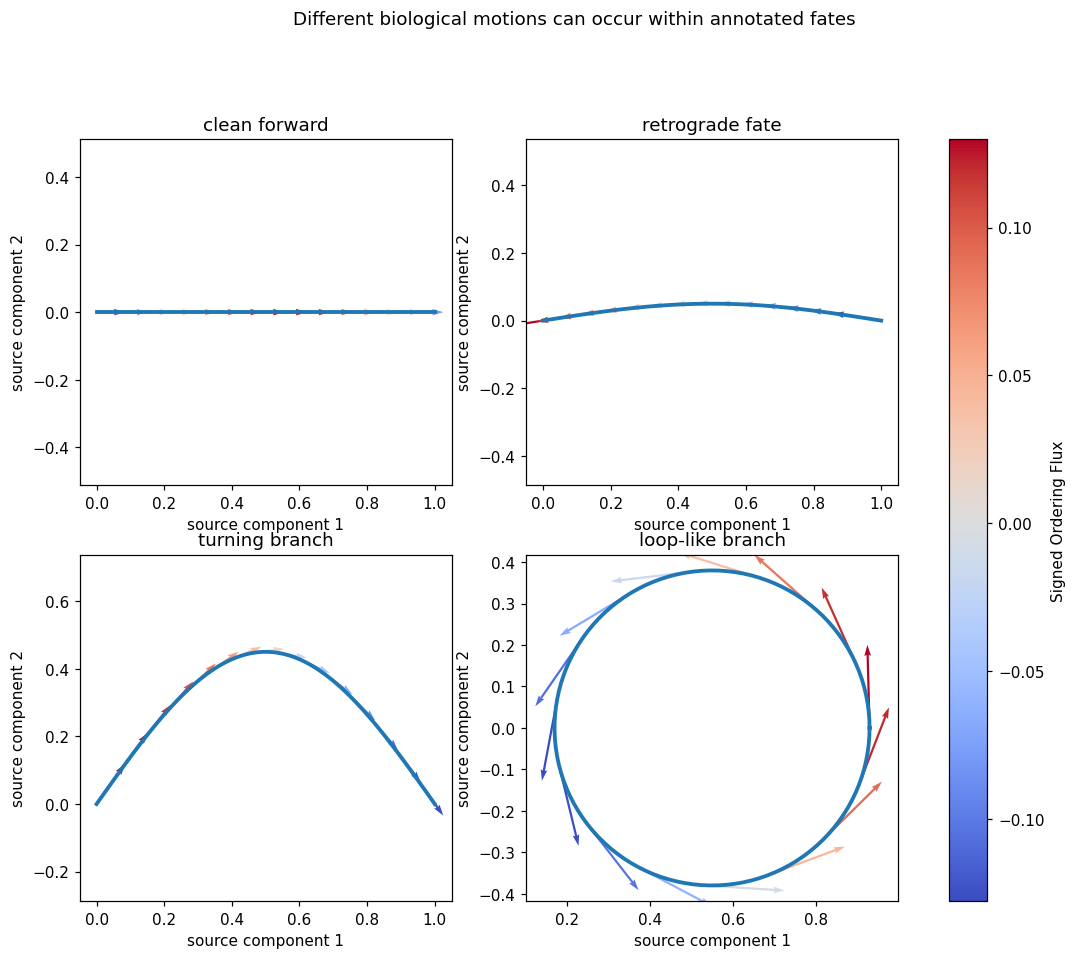
Arrows show local motion in the source manifold. The branch annotation does not guarantee that every arrow points toward larger ordering values.

fig, axes = plt.subplots(2, 2, figsize=(12, 9))
for axis, (name, values) in zip(axes.ravel(), archetypes.items()):
    x = values["x"]
    y = values["y"]
    dx = np.gradient(x)
    dy = np.gradient(y)
    if name == "retrograde fate":
        dx = -np.abs(dx)
        dy = -dy
    sample = np.arange(0, len(t), 8)
    axis.plot(x, y, linewidth=2.5)
    arrows = axis.quiver(
        x[sample],
        y[sample],
        dx[sample],
        dy[sample],
        values["flux"][sample],
        cmap="coolwarm",
        angles="xy",
        scale_units="xy",
        scale=0.10,
        width=0.006,
    )
    axis.set_title(name)
    axis.set_xlabel("source component 1")
    axis.set_ylabel("source component 2")
    axis.set_aspect("equal", adjustable="datalim")
fig.colorbar(arrows, ax=axes.ravel().tolist(), label="Signed Ordering Flux")
fig.suptitle("Different biological motions can occur within annotated fates", y=1.01)
plt.show()

5. Identity, resolution, and progression along ordering

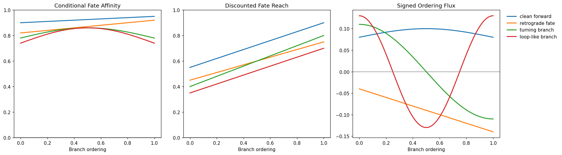
High affinity does not imply positive progression. The turning and loop-like examples keep a coherent future identity while SOF changes sign.

fig, axes = plt.subplots(1, 3, figsize=(17, 4.8))
for name, values in archetypes.items():
    axes[0].plot(t, values["affinity"], linewidth=2, label=name)
    axes[1].plot(t, values["reach"], linewidth=2, label=name)
    axes[2].plot(t, values["flux"], linewidth=2, label=name)
axes[0].set_title("Conditional Fate Affinity")
axes[1].set_title("Discounted Fate Reach")
axes[2].set_title("Signed Ordering Flux")
for axis in axes:
    axis.set_xlabel("Branch ordering")
    axis.axhline(0, color="0.5", linewidth=1)
axes[0].set_ylim(0, 1)
axes[1].set_ylim(0, 1)
axes[2].legend(frameon=False, bbox_to_anchor=(1.02, 1), loc="upper left")
fig.tight_layout()
plt.show()

6. A two-axis interpretation map

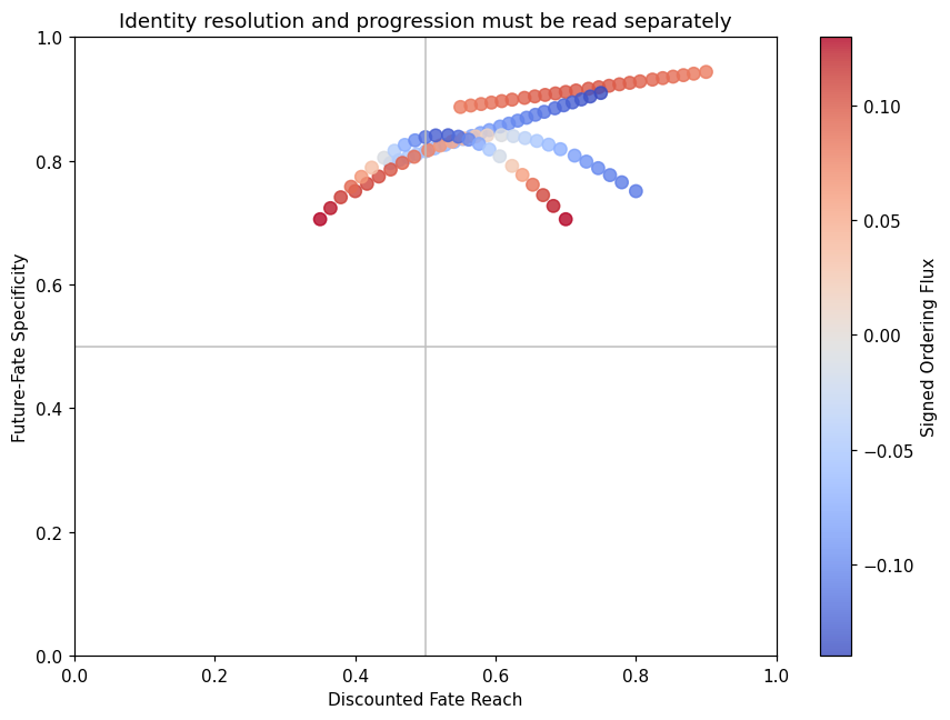
DFR and FFS answer different questions. Color adds SOF:

• upper right: resolved and specific;

• upper left: specific but weakly reached;

• lower right: reached but fate-ambiguous;

• lower left: unresolved and ambiguous.

Negative color does not invalidate a point; it indicates retrograde motion.

rows = []
for name, values in archetypes.items():
    for index in np.linspace(0, len(t) - 1, 24).astype(int):
        rows.append(
            {
                "archetype": name,
                "reach": values["reach"][index],
                "specificity": values["specificity"][index],
                "flux": values["flux"][index],
            }
        )
map_table = pd.DataFrame(rows)

fig, ax = plt.subplots(figsize=(8, 6))
scatter = ax.scatter(
    map_table["reach"],
    map_table["specificity"],
    c=map_table["flux"],
    cmap="coolwarm",
    s=55,
    alpha=0.8,
)
ax.axvline(0.5, color="0.75", linewidth=1)
ax.axhline(0.5, color="0.75", linewidth=1)
ax.set_xlim(0, 1)
ax.set_ylim(0, 1)
ax.set_xlabel("Discounted Fate Reach")
ax.set_ylabel("Future-Fate Specificity")
ax.set_title("Identity resolution and progression must be read separately")
fig.colorbar(scatter, ax=ax, label="Signed Ordering Flux")
fig.tight_layout()
plt.show()

7. Branch-relative velocity-angle profiles

For a terminal branch, (0^:nbsphinx-math:circ) is outward, (180^:nbsphinx-math:circ) is inward, and (\pm90`^:nbsphinx-math:circ`) is transverse. These profiles are display diagnostics; they do not replace DFFP.

The synthetic distributions below show how clean, retrograde, turning, and loop-like branches appear when referenced to their own branch axes.

angle_samples = {
    "clean forward": rng.normal(0.0, 12.0, 500),
    "retrograde fate": rng.normal(180.0, 14.0, 500),
    "turning branch": np.r_[
        rng.normal(35.0, 18.0, 250),
        rng.normal(120.0, 22.0, 250),
    ],
    "loop-like branch": rng.uniform(-180.0, 180.0, 500),
}

fig, axes = plt.subplots(
    2,
    2,
    figsize=(11, 10),
    subplot_kw={"projection": "polar"},
)
bins = np.linspace(-np.pi, np.pi, 25)
for axis, (name, degrees) in zip(axes.ravel(), angle_samples.items()):
    radians = np.deg2rad(((degrees + 180) % 360) - 180)
    counts, edges = np.histogram(radians, bins=bins)
    centers = 0.5 * (edges[:-1] + edges[1:])
    width = np.diff(edges)
    axis.bar(centers, counts / max(counts.max(), 1), width=width, alpha=0.8)
    axis.set_theta_zero_location("E")
    axis.set_theta_direction(1)
    axis.set_title(name, pad=18)
    axis.set_yticklabels([])
fig.suptitle("Branch-relative display-velocity profiles", y=1.01)
fig.tight_layout()
plt.show()

8. Anchor diagnostics are context, not monotonicity gates

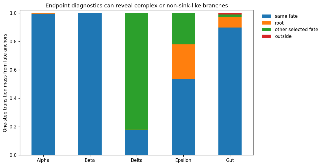
The pancreas benchmark contained strong sink-like Alpha and Beta endpoints, whereas Delta and Epsilon retained substantial transition mass toward other states. Gut in the Schwann benchmark remained annotation-coherent but showed retrograde SOF.

The stacked bars below illustrate the diagnostic quantities that should be reported.

anchor_example = pd.DataFrame(
    {
        "same fate": [0.996, 1.000, 0.178, 0.534, 0.898],
        "root": [0.001, 0.000, 0.001, 0.245, 0.074],
        "other selected fate": [0.003, 0.000, 0.821, 0.220, 0.018],
        "outside": [0.000, 0.000, 0.000, 0.001, 0.010],
    },
    index=["Alpha", "Beta", "Delta", "Epsilon", "Gut"],
)
ax = anchor_example.plot(
    kind="bar",
    stacked=True,
    figsize=(10, 5.2),
    ylabel="One-step transition mass from late anchors",
    title="Endpoint diagnostics can reveal complex or non-sink-like branches",
)
ax.set_ylim(0, 1.02)
ax.legend(frameon=False, bbox_to_anchor=(1.02, 1), loc="upper left")
plt.xticks(rotation=0)
plt.tight_layout()
plt.show()
anchor_example

	same fate	root	other selected fate	outside
Alpha	0.996	0.001	0.003	0.000
Beta	1.000	0.000	0.000	0.000
Delta	0.178	0.001	0.821	0.000
Epsilon	0.534	0.245	0.220	0.001
Gut	0.898	0.074	0.018	0.010

9. Summarizing real scCS results

def summarize_branches(result, annotations):
    table = pd.DataFrame(
        {
            "annotation": np.asarray(annotations).astype(str),
            "DFR": result.discounted_fate_reach,
            "FFS": result.future_fate_specificity,
            "RC": result.resolved_commitment,
            "SOF": result.signed_ordering_flux,
        }
    )
    for fate_index, fate in enumerate(result.fate_names):
        table[f"CFA:{fate}"] = result.conditional_fate_affinity[:, fate_index]
    return table.groupby("annotation", observed=True).agg(
        n_cells=("DFR", "size"),
        mean_DFR=("DFR", "mean"),
        mean_FFS=("FFS", "mean"),
        mean_RC=("RC", "mean"),
        mean_SOF=("SOF", "mean"),
        forward_fraction=("SOF", lambda values: float(np.mean(values > 0))),
    )


def add_ordering_thirds(frame, ordering_column):
    output = frame.copy()
    output["ordering_third"] = "middle"
    for annotation, indices in output.groupby("annotation", observed=True).groups.items():
        ranks = output.loc[indices, ordering_column].rank(method="first", pct=True)
        output.loc[indices, "ordering_third"] = pd.cut(
            ranks,
            bins=[0, 1 / 3, 2 / 3, 1],
            labels=["early", "middle", "late"],
            include_lowest=True,
        ).astype(str)
    return output

10. Interpretation checklist

1. Inspect the native velocity field before the star.

2. Read CFA, DFR, FFS, and RC before display-space arrows.

3. Interpret SOF independently from fate identity.

4. Use ordering thirds to distinguish uniformly retrograde motion from a turn or loop.

5. Report weak sink behavior, but do not relabel it as a software failure.

6. Restrict hard dominant-fate labels when specificity or the probability margin is low.

7. Remember that display velocity profiles are qualitative QC and DFFP remains the scientific score.