Mathematical framework
Notation
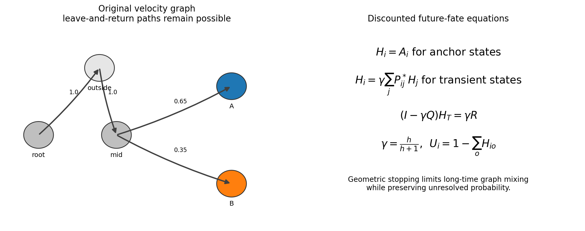
Let \(P\in\mathbb{R}^{N\times N}\) be a non-negative row-stochastic transition matrix from the RNA-velocity graph. Let \(S\) denote the selected root-plus-fate cells, and let \(A\in\{0,1\}^{N\times O}\) identify the anchor states for \(O\) selected and optional competing outcomes.
Discounted Future-Fate Propagation
Anchor rows are made absorbing to form \(P^*\). Before each transition the process stops with probability \(1-\gamma\), where
The expected number of continued transitions is \(\gamma/(1-\gamma)=h\),
so effective_horizon=h is an interpretable graph scale rather than physical
time.
For an anchor state, the outcome vector equals its anchor indicator. For a transient state,
Partitioning the absorbing chain into transient-to-transient block \(Q\) and transient-to-anchor block \(R\) gives
scCS uses sparse direct solution for modest graphs and sparse fixed-point iteration for large graphs. The unresolved probability is
Selected-fate metrics
Let \(p_{if}\) denote the DFFP probability for selected fate \(f\). Discounted Fate Reach is
Conditional Fate Affinity is defined when \(R_i\) exceeds the configured minimum reach:
Normalized future-fate entropy and Future-Fate Specificity are
Resolved Commitment is
CFA describes identity, DFR describes resolution, FFS describes decisiveness, and RC combines resolution with decisiveness. These values should be reported separately rather than replacing them with one composite.
Signed Ordering Flux
Let \(s_i\) be the supplied ordering. The one-step selected-path coverage is
Conditioning transitions on remaining inside the selected furcation gives
Signed Ordering Flux is
Positive \(g_i\) is forward, negative \(g_i\) is retrograde, and values near zero may represent stationary, mixed, turning, or loop-like motion. The support-weighted flux \(c_ig_i\) is also available when outside-path mass should reduce the contribution.
Endpoint anchors
For each fate, scCS selects late cells within that annotated fate using the ordering quantile and a minimum anchor count. Anchor diagnostics report transition mass to the same fate, root, other selected fates, and outside the selected path. Non-sink-like anchors are warnings for interpretation, not automatic failures.
Instantaneous mode
For selected star coordinates \(y_i\) and retained normalized transition weights \(\widetilde{P}_{ij}\), instantaneous mode computes
The fate-directed component is compared with ideal regular-simplex directions. For \(K\) fates, these directions satisfy
Cosine-softmax affinity is then
This mode measures immediate local direction in the supervised geometry. It is not the same as DFFP and should not be interpreted as long-term fate probability.
Condition inference
PairScorer and MultiScorer use one pooled scientific model and aggregate cell metrics within genuine biological replicates. Formal inference permutes replicate labels, not cell labels. Hierarchical bootstrap resamples replicates first and cells within replicate second. This preserves the experimental unit and avoids pseudoreplication.
Parameter interpretation
effective_horizon controls graph depth, anchor_quantile controls how
late endpoint anchors are, min_anchor_cells prevents tiny anchor sets, and
min_reach controls when CFA is considered defined. A defensible analysis
reports sensitivity across plausible horizons and anchor quantiles.