RegVelo Schwann SingleScorer tutorial
This notebook reproduces the curated neural-crest/Schwann furcation:
Common Progenitor → Gut, Gut neuron, ChC.
The primary ordering is inverse CytoTRACE pseudotime because it was the coherent benchmark-specific ordering in independent validation. It is not a universal scCS default. Gut is allowed to show retrograde velocity toward Common Progenitor.
Execution provenance. The displayed outputs were generated with scCS 0.8.0.dev33. Version 0.8.0.dev34 changes documentation and tutorial explanation only; the scientific calculations are unchanged.
1. Installation, versions, and reproducibility
[1]:
from __future__ import annotations
import warnings

from pathlib import Path
import importlib.metadata as importlib_metadata
import platform
import sys

import matplotlib.pyplot as plt
import numpy as np
import pandas as pd
import scanpy as sc
import scvelo as scv
from scipy.spatial.distance import jensenshannon
from scipy.stats import spearmanr

import scCS

SEED = 20260714
N_JOBS = 1
sc.settings.verbosity = 2
scv.settings.verbosity = 2
sc.set_figure_params(dpi=100, facecolor="white")

print("Python", sys.version.split()[0])
print("Platform", platform.platform())
print("scCS", scCS.__version__)
print("Scanpy", importlib_metadata.version("scanpy"))
print("scVelo", scv.__version__)

OUTPUT_DIR = Path("tutorial_outputs/schwann_single")
OUTPUT_DIR.mkdir(parents=True, exist_ok=True)

# Hide known warnings emitted by optional upstream dependencies. These do not
# change the scCS calculation and would otherwise distract from the tutorial.
warnings.filterwarnings(
    "ignore",
    message=r"This process .* is multi-threaded, use of fork\(\) may lead to deadlocks.*",
    category=DeprecationWarning,
)
warnings.filterwarnings(
    "ignore",
    category=DeprecationWarning,
    module=r"cellrank\..*",
)
Python 3.12.13
Platform Linux-6.6.114.1-microsoft-standard-WSL2-x86_64-with-glibc2.39
scCS 0.8.0.dev33
Scanpy 1.11.5
scVelo 0.3.4
2. Load RegVelo Schwann, reproduce the curated clusters, and fit velocity
The Schwann tutorials use dynamical RNA velocity as the primary model. The dataset is loaded directly from RegVelo and the velocity model is fitted in the original expression/PCA manifold. No tutorial cache is assumed.
The inverse-CytoTRACE coordinate is used only as the validated ordering for this particular furcation; scCS does not prescribe it as a universal pseudotime.
[2]:
def clear_velocity_outputs(adata, *, clear_dynamics=False):
    """Remove stale velocity fields before fitting a requested model."""
    for key in ("velocity", "velocity_u", "velocity_variance"):
        adata.layers.pop(key, None)
    for key in ("velocity_graph", "velocity_graph_neg", "velocity_params"):
        adata.uns.pop(key, None)
    for key in (
        "velocity_self_transition",
        "root_cells",
        "end_points",
        "velocity_pseudotime",
        "latent_time",
    ):
        if key in adata.obs:
            del adata.obs[key]
    if clear_dynamics:
        for key in list(adata.var.columns):
            if str(key).startswith("fit_"):
                del adata.var[key]
        for key in list(adata.layers):
            if str(key).startswith("fit_"):
                del adata.layers[key]
        adata.uns.pop("recover_dynamics", None)


def ensure_pca_neighbors_moments(
    adata,
    *,
    n_pcs=30,
    n_neighbors=30,
    preserve_existing_neighbors=False,
):
    """Create the unbiased PCA neighbor graph used by RNA velocity."""
    if "X_pca" not in adata.obsm:
        n_comps = min(n_pcs, adata.n_obs - 1, adata.n_vars - 1)
        sc.pp.pca(adata, n_comps=n_comps)
    if "neighbors" not in adata.uns or not preserve_existing_neighbors:
        sc.pp.neighbors(
            adata,
            n_neighbors=min(n_neighbors, adata.n_obs - 1),
            n_pcs=min(n_pcs, adata.obsm["X_pca"].shape[1]),
            use_rep="X_pca",
            random_state=SEED,
        )
    if not {"Ms", "Mu"}.issubset(adata.layers):
        scv.pp.moments(adata, n_neighbors=None, n_pcs=None)
    if "X_umap" not in adata.obsm:
        sc.tl.umap(adata, random_state=SEED)


def resolve_present_genes(adata, candidates):
    """Resolve gene symbols case-insensitively and report missing markers."""
    lookup = {str(gene).lower(): str(gene) for gene in adata.var_names}
    resolved, missing = [], []
    for candidate in candidates:
        match = lookup.get(str(candidate).lower())
        if match is None:
            missing.append(str(candidate))
        elif match not in resolved:
            resolved.append(match)
    return resolved, missing


def row_js(left, right):
    """Row-wise Jensen-Shannon divergence with base-2 logarithms."""
    return np.asarray(
        [jensenshannon(a, b, base=2.0) ** 2 for a, b in zip(left, right)],
        dtype=float,
    )


def ordering_thirds(values):
    """Return stable early/middle/late labels for a continuous coordinate."""
    series = pd.Series(np.asarray(values, dtype=float))
    ranked = series.rank(method="first")
    return (
        pd.qcut(
            ranked,
            q=3,
            labels=["early", "middle", "late"],
            duplicates="drop",
        )
        .astype(str)
        .to_numpy()
    )
[3]:
import regvelo as rgv

SCHWANN_CLUSTER_ANNOTATION = {
    "15": "Common Progenitor",
    "5": "Common Progenitor",
    "16": "Gut",
    "12": "Gut neuron",
    "8": "ChC",
    "6": "ChC",
}
VELOCITY_MODEL = "dynamical"
RECOVER_DYNAMICS_MAX_ITER = 20


def prepare_schwann_annotations(adata):
    """Reproduce the curated Schwann furcation and inverse-CytoTRACE ordering."""
    if "neighbors" not in adata.uns or "connectivities" not in adata.obsp:
        raise RuntimeError("The original RegVelo neighbor graph is required.")

    if "sccs_leiden" not in adata.obs:
        sc.tl.leiden(
            adata,
            resolution=1.0,
            random_state=0,
            key_added="sccs_leiden",
        )

    leiden = adata.obs["sccs_leiden"].astype(str)
    adata.obs["cell_type_new"] = (
        leiden.map(SCHWANN_CLUSTER_ANNOTATION).fillna("Other").astype("category")
    )

    required = ("Common Progenitor", "Gut", "Gut neuron", "ChC")
    counts = adata.obs["cell_type_new"].astype(str).value_counts().reindex(required, fill_value=0)
    if np.any(counts <= 0):
        raise ValueError(
            f"The curated furcation was not reproduced. Observed counts: {counts.to_dict()}"
        )

    cytotrace = pd.to_numeric(adata.obs["CytoTRACE"], errors="coerce").to_numpy(float)
    finite = np.isfinite(cytotrace)
    lower = float(np.nanmin(cytotrace))
    upper = float(np.nanmax(cytotrace))
    inverse = np.full(adata.n_obs, np.nan, dtype=float)
    inverse[finite] = 1.0 - (cytotrace[finite] - lower) / (upper - lower)
    adata.obs["inverse_cytotrace_pseudotime"] = inverse


# Load the public RegVelo Schwann dataset and reproduce the curated annotations.
adata = rgv.datasets.schwann()
adata.var_names_make_unique()
prepare_schwann_annotations(adata)

# Fit the dynamical model in the original expression/PCA manifold.
# This is the primary Schwann model used by the tutorials.
ensure_pca_neighbors_moments(
    adata,
    n_pcs=30,
    n_neighbors=30,
    preserve_existing_neighbors=True,
)
clear_velocity_outputs(adata, clear_dynamics=True)
scv.tl.recover_dynamics(
    adata,
    max_iter=RECOVER_DYNAMICS_MAX_ITER,
    n_jobs=N_JOBS,
)
scv.tl.velocity(adata, mode="dynamical")
scv.tl.velocity_graph(adata, n_jobs=N_JOBS)
prepare_schwann_annotations(adata)

print(adata)
display(adata.obs["cell_type_new"].astype(str).value_counts().to_frame("n_cells"))
try downloading from url
https://drive.usercontent.google.com/download?id=1ZpG1gz0jjPNuXc_bsz3XInVtHooHU02M&export=download&authuser=1&confirm=t&uuid=eeed9d4b-c938-40c9-af24-b248fd29e161&at=AN8xHoqO3RF2oroUCmn7jFURR16T:1754642525195
... this may take a while but only happens once
creating directory data/schwann/ for saving data
running Leiden clustering
    finished (0:00:01)
recovering dynamics (using 1/24 cores)
    finished (0:24:07)
computing velocities
    finished (0:00:14)
computing velocity graph (using 1/24 cores)
    finished (0:00:17)
AnnData object with n_obs × n_vars = 8821 × 1150
    obs: 'plates', 'devtime', 'location', 'n_genes_by_counts', 'total_counts', 'total_counts_ERCC', 'pct_counts_ERCC', 'doublet_scores', 'leiden', 'CytoTRACE', 'Gut_neuron', 'Sensory', 'Symp', 'enFib', 'ChC', 'Gut_glia', 'NCC', 'Mesenchyme', 'Melanocytes', 'SatGlia', 'SC', 'BCC', 'conflict', 'assignments', 'batch', 'initial_size_unspliced', 'initial_size_spliced', 'initial_size', 'n_counts', 'sccs_leiden', 'cell_type_new', 'inverse_cytotrace_pseudotime', 'velocity_self_transition'
    var: 'ERCC', 'n_cells_by_counts', 'mean_counts', 'pct_dropout_by_counts', 'total_counts', 'n_cells', 'm', 'v', 'n_obs', 'res', 'lp', 'lpa', 'qv', 'highly_variable', 'Accession', 'Chromosome', 'End', 'Start', 'Strand', 'TF', 'means', 'dispersions', 'dispersions_norm', 'velocity_genes', 'fit_alpha', 'fit_beta', 'fit_gamma', 'fit_t_', 'fit_scaling', 'fit_std_u', 'fit_std_s', 'fit_likelihood', 'fit_u0', 'fit_s0', 'fit_pval_steady', 'fit_steady_u', 'fit_steady_s', 'fit_variance', 'fit_alignment_scaling', 'fit_r2'
    uns: 'assignments_colors', 'devtime_colors', 'hvg', 'leiden', 'leiden_colors', 'leiden_sizes', 'location_colors', 'log1p', 'neighbors', 'network', 'paga', 'regulators', 'skeleton', 'targets', 'umap', 'sccs_leiden', 'recover_dynamics', 'velocity_params', 'velocity_graph', 'velocity_graph_neg'
    obsm: 'X_diff', 'X_pca', 'X_umap'
    varm: 'loss'
    layers: 'GEX', 'Ms', 'Mu', 'ambiguous', 'matrix', 'palantir_imp', 'scaled', 'spanning', 'spliced', 'unspliced', 'fit_t', 'fit_tau', 'fit_tau_', 'velocity', 'velocity_u'
    obsp: 'connectivities', 'distances'
| n_cells | |
|---|---|
| cell_type_new | |
| Other | 6845 |
| ChC | 762 |
| Common Progenitor | 675 |
| Gut neuron | 294 |
| Gut | 245 |
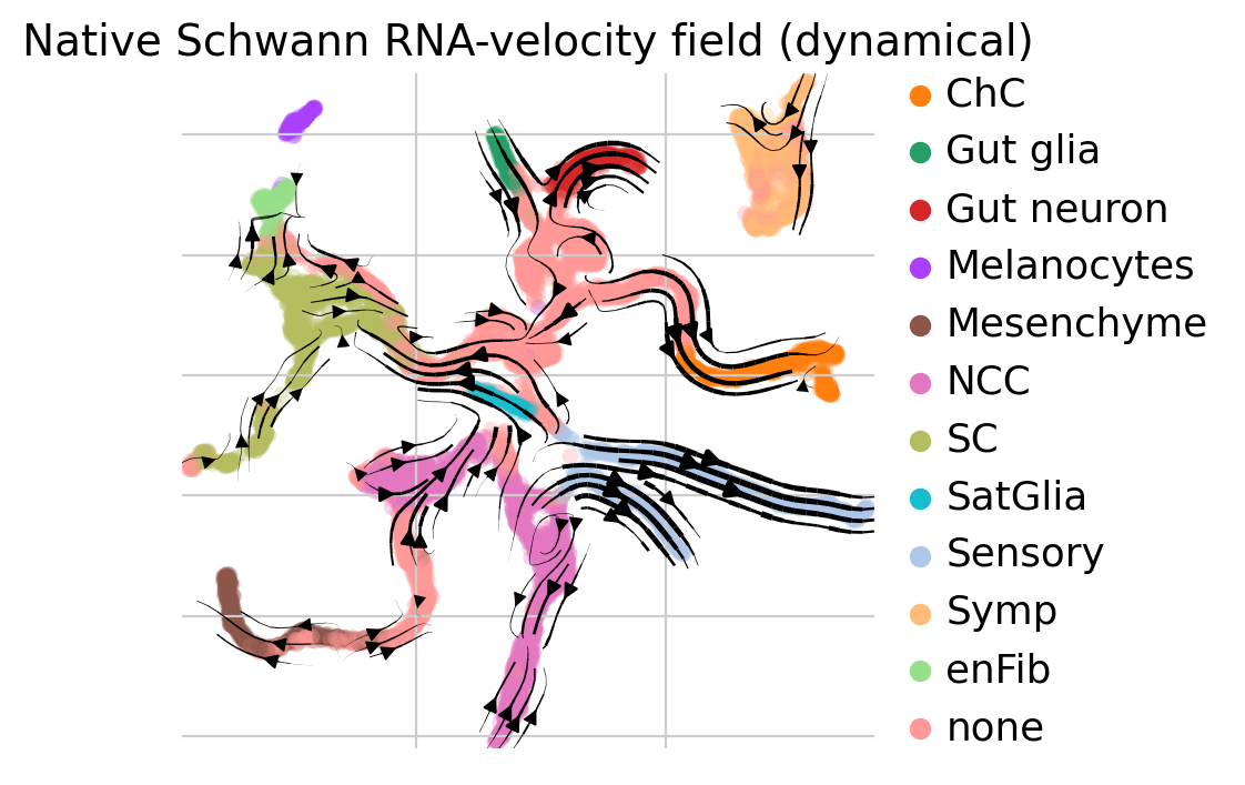
3. Inspect the native manifold and curated topology
[4]:
selected_labels = ["Common Progenitor", "Gut", "Gut neuron", "ChC"]
selected_mask_full = adata.obs["cell_type_new"].astype(str).isin(selected_labels)
display(
    adata.obs.loc[
        selected_mask_full,
        ["cell_type_new", "inverse_cytotrace_pseudotime"],
    ]
    .groupby("cell_type_new", observed=True)
    .agg(["count", "median", "min", "max"])
)

color_key = "assignments" if "assignments" in adata.obs else "cell_type_new"
scv.pl.velocity_embedding_stream(
    adata,
    basis="umap",
    color=color_key,
    legend_loc="right margin",
    title=f"Native Schwann RNA-velocity field ({VELOCITY_MODEL})",
)
| inverse_cytotrace_pseudotime | ||||
|---|---|---|---|---|
| count | median | min | max | |
| cell_type_new | ||||
| ChC | 762 | 0.607434 | 0.276986 | 0.829939 |
| Common Progenitor | 675 | 0.420570 | 0.267821 | 0.853360 |
| Gut | 245 | 0.797352 | 0.459267 | 0.875764 |
| Gut neuron | 294 | 0.525967 | 0.336049 | 0.779022 |
computing velocity embedding
    finished (0:00:01)
4. Define the supervised furcation and run preflight diagnostics
[5]:
ROOT = "Common Progenitor"
FATES = ["Gut", "Gut neuron", "ChC"]
ORDERING_KEY = "inverse_cytotrace_pseudotime"

scorer = scCS.SingleScorer(
    adata,
    root=ROOT,
    branches=FATES,
    obs_key="cell_type_new",
)
preflight = scorer.preflight(ordering_metric=ORDERING_KEY, check_velocity=True)
preflight.display()
preflight.raise_for_errors()
scorer.build_embedding(
    ordering_metric=ORDERING_KEY,
    write_to_adata=True,
)
| level | code | message | value | |
|---|---|---|---|---|
| 0 | info | furcation_valid | Root and terminal annotations are valid. | 1976.000000 |
| 1 | info | root_cells | Root population contains 675 cells. | 675.000000 |
| 2 | info | terminal_Gut | Terminal 'Gut' contains 245 cells. | 245.000000 |
| 3 | info | terminal_Gut neuron | Terminal 'Gut neuron' contains 294 cells. | 294.000000 |
| 4 | info | terminal_ChC | Terminal 'ChC' contains 762 cells. | 762.000000 |
| 5 | info | ordering_valid | Ordering metric is finite and non-constant amo... | 1.000000 |
| 6 | info | ordering_resolution | Root ordering has 337 unique values across 675... | 0.499259 |
| 7 | info | velocity_available | Velocity information is available. | NaN |
[scCS] Scientific star built for 1976 cells in 3 dimensions.
       Root radial clipping: 0.050 low / 0.050 high
       Terminal scientific coordinates: fixed equal-radius simplex vertices (radius=1.000).
[5]:
<scCS.single.SingleScorer at 0x70725c6a1a00>
5. Fit discounted future-fate scoring
[6]:
FUTURE_OPTIONS = {
    "effective_horizon": 64,
    "anchor_quantile": 0.90,
    "min_anchor_cells": 10,
    "progression_scale": "rank",
    "committed_reach_threshold": 0.25,
    "committed_specificity_threshold": 0.25,
}
scorer.fit(
    scoring_mode="future_fate",
    future_fate_options=FUTURE_OPTIONS,
)
result = scorer.score(write_to_adata=True)
display(pd.Series(result.summary(), name="value").to_frame())
anchor_diagnostics = result.anchor_diagnostics_frame()
display(anchor_diagnostics)
anchor_diagnostics.to_csv(OUTPUT_DIR / "anchor_diagnostics.csv", index=False)
scCS FutureFateScoreResult
  Furcation: Common Progenitor -> ['Gut', 'Gut neuron', 'ChC']
  Effective horizon: 64 (gamma=0.984615)
  Cells: 1976 selected; 675 root
  Root affinity coverage: 1.000
  Root mean future-fate reach: 0.156
  Root mean future-fate entropy: 0.877
  Root mean future-fate specificity: 0.123
  Root mean reach-supported specificity: 0.025
  Root mean unresolved probability: 0.844
  Root mean signed progression: 0.020
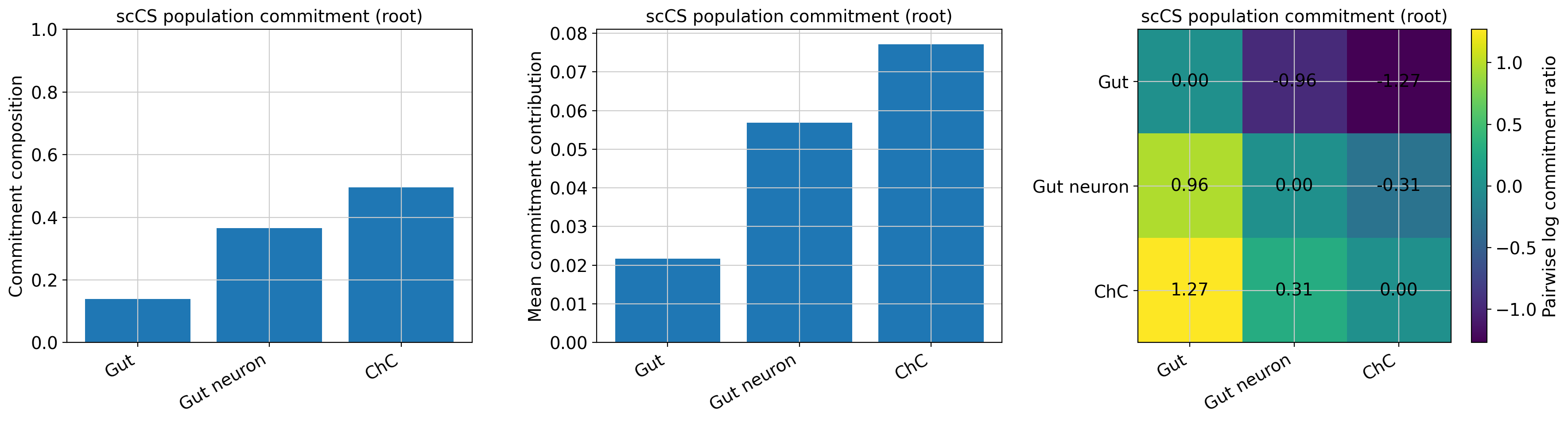
  Root future-fate composition: Gut=0.139, Gut neuron=0.365, ChC=0.496
  Solver: direct; iterations=1; residual=3.315e-15
scCS FutureFateScoreResult
  Furcation: Common Progenitor -> ['Gut', 'Gut neuron', 'ChC']
  Effective horizon: 64 (gamma=0.984615)
  Cells: 1976 selected; 675 root
  Root affinity coverage: 1.000
  Root mean future-fate reach: 0.156
  Root mean future-fate entropy: 0.877
  Root mean future-fate specificity: 0.123
  Root mean reach-supported specificity: 0.025
  Root mean unresolved probability: 0.844
  Root mean signed progression: 0.020
  Root future-fate composition: Gut=0.139, Gut neuron=0.365, ChC=0.496
  Solver: direct; iterations=1; residual=3.315e-15
| value | |
|---|---|
| 0 | scCS FutureFateScoreResult\n Furcation: Commo... |
| fate | n_anchors | mean_transition_to_same_fate_population | mean_transition_to_root | mean_transition_to_other_selected_fates | mean_transition_outside_selected_path | mean_signed_progression | forward_fraction | |
|---|---|---|---|---|---|---|---|---|
| 0 | Gut | 26 | 0.919012 | 0.046293 | 0.000000 | 0.034694 | -0.112502 | 0.0 |
| 1 | Gut neuron | 30 | 0.879802 | 0.000610 | 0.009397 | 0.110191 | -0.123093 | 0.0 |
| 2 | ChC | 79 | 0.948219 | 0.000000 | 0.000000 | 0.051781 | -0.084801 | 0.0 |
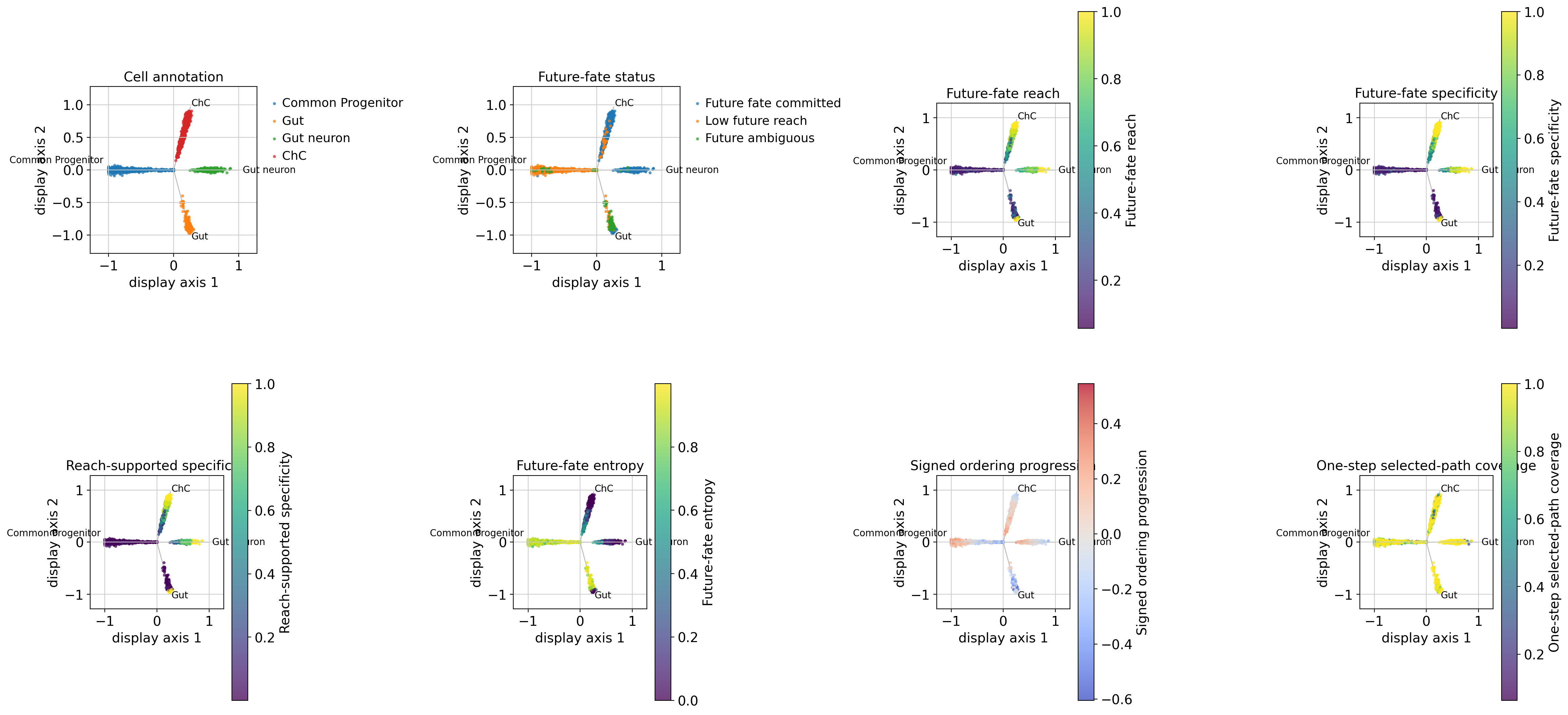
6. Core star dashboard
[7]:
fig, axes = plt.subplots(2, 4, figsize=(23, 11))
scorer.plot_star(result, color_by="population", title="Cell annotation", ax=axes[0, 0])
scorer.plot_star(result, color_by="status", title="Future-fate status", ax=axes[0, 1])
scorer.plot_star(result, color_by="future_fate_reach", title="Future-fate reach", ax=axes[0, 2])
scorer.plot_star(
    result,
    color_by="future_fate_specificity",
    title="Future-fate specificity",
    ax=axes[0, 3],
)
scorer.plot_star(
    result,
    color_by="reach_supported_specificity",
    title="Reach-supported specificity",
    ax=axes[1, 0],
)
scorer.plot_star(result, color_by="future_fate_entropy", title="Future-fate entropy", ax=axes[1, 1])
scorer.plot_star(
    result,
    color_by="signed_progression",
    title="Signed ordering progression",
    cmap="coolwarm",
    ax=axes[1, 2],
)
scorer.plot_star(
    result,
    color_by="selected_path_coverage",
    title="One-step selected-path coverage",
    ax=axes[1, 3],
)
fig.tight_layout()
fig.savefig(OUTPUT_DIR / "core_star_dashboard.png", dpi=200, bbox_inches="tight")
plt.show()
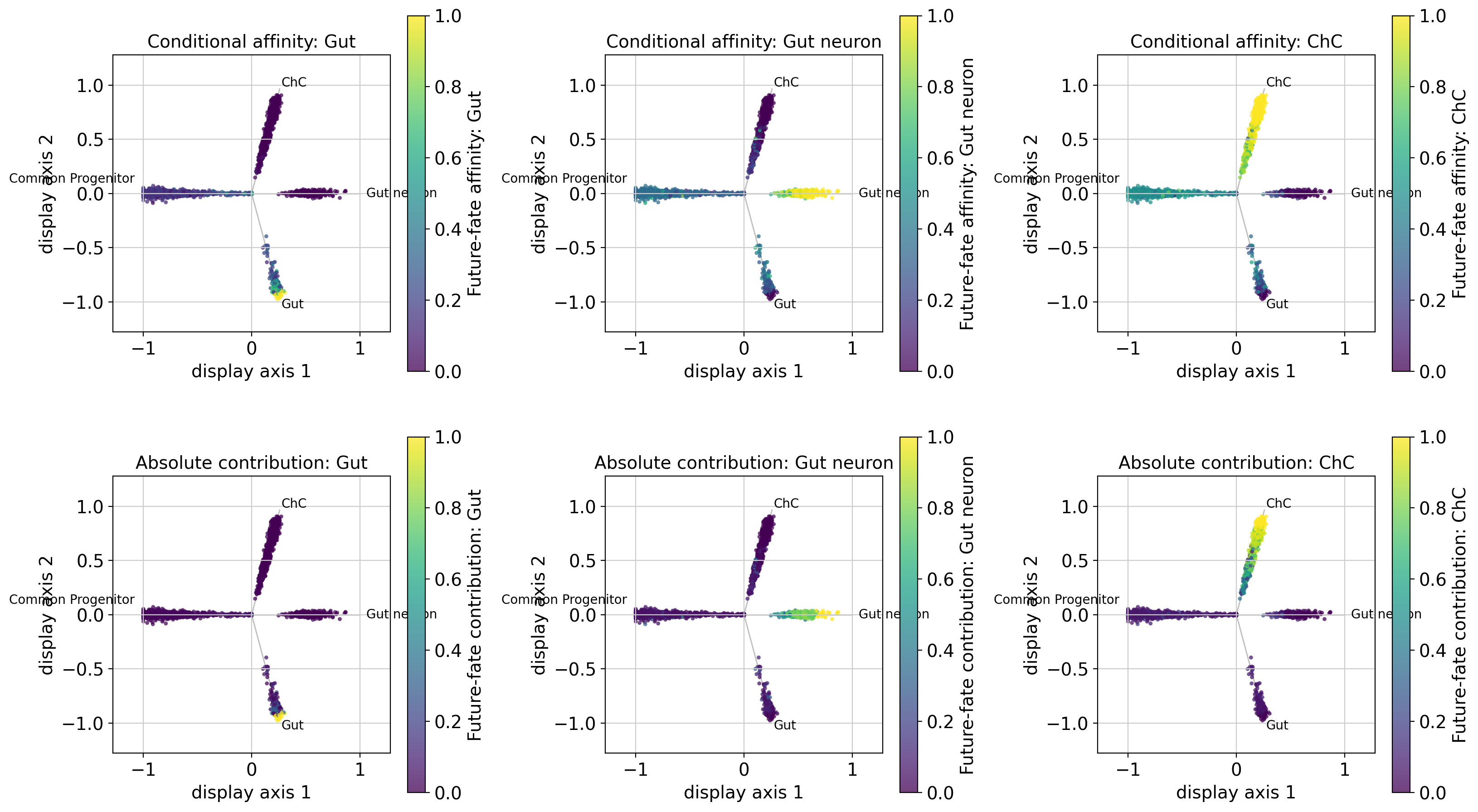
7. Fate-specific affinity and contribution
[8]:
fig, axes = plt.subplots(2, len(FATES), figsize=(5.5 * len(FATES), 9.5))
for column, fate in enumerate(FATES):
    scorer.plot_star(
        result,
        color_by=f"future_fate_affinity:{fate}",
        title=f"Conditional affinity: {fate}",
        ax=axes[0, column],
    )
    scorer.plot_star(
        result,
        color_by=f"future_fate_contribution:{fate}",
        title=f"Absolute contribution: {fate}",
        ax=axes[1, column],
    )
fig.tight_layout()
fig.savefig(OUTPUT_DIR / "fate_affinity_and_contribution.png", dpi=200, bbox_inches="tight")
plt.show()
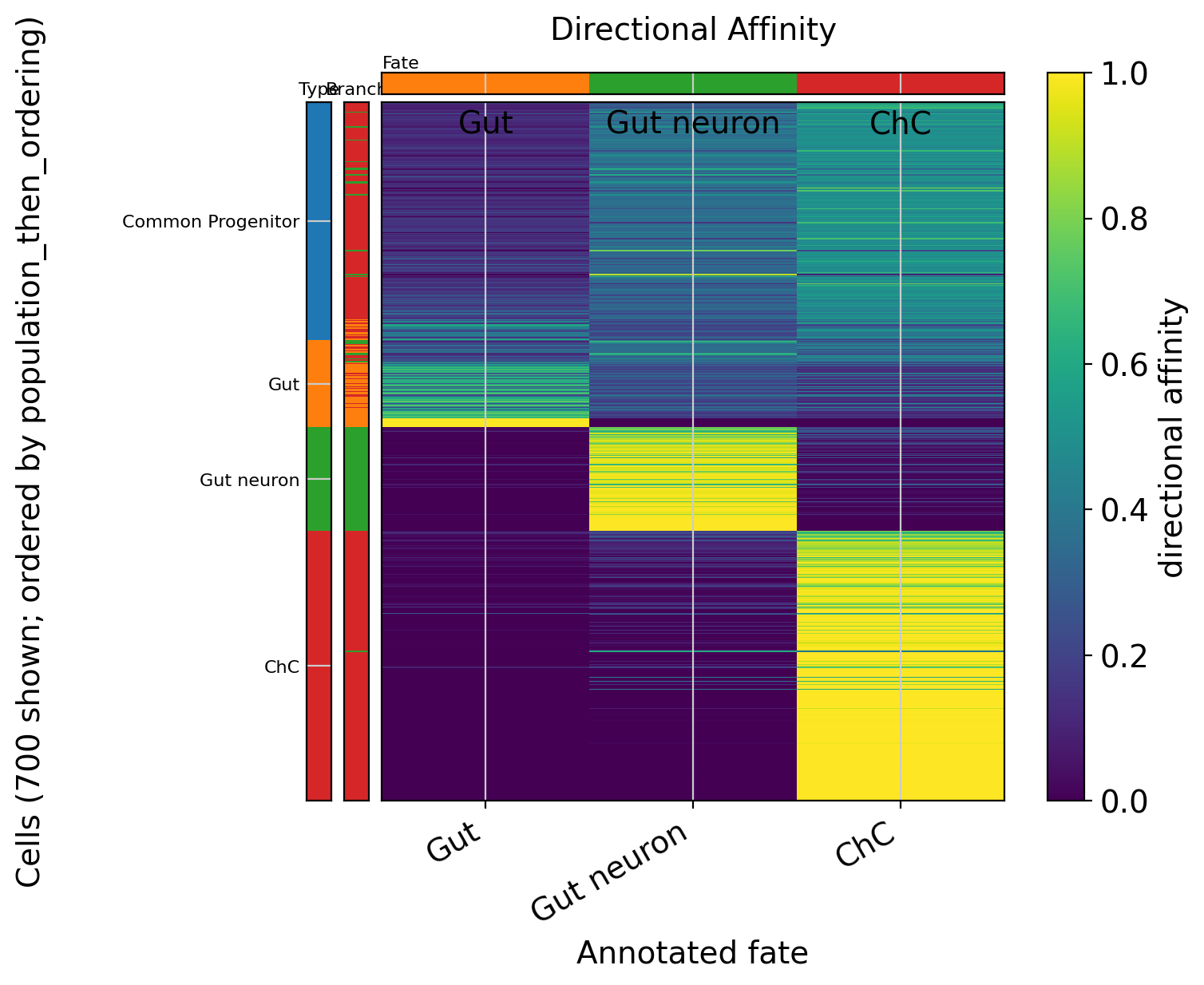
8. Heatmaps with cell-type and dominant-affinity strips
[9]:
affinity_fig = scorer.plot_commitment_heatmap(
    result,
    metric="future_fate_affinity",
    population="all",
    sort_by="population_then_ordering",
    row_annotation=("population", "dominant_affinity"),
    show_fate_strip=True,
    max_cells=700,
)
affinity_fig.savefig(OUTPUT_DIR / "future_fate_affinity_heatmap.png", dpi=200, bbox_inches="tight")
plt.show()

contribution_fig = scorer.plot_commitment_heatmap(
    result,
    metric="future_fate_contribution",
    population="all",
    sort_by="population_then_ordering",
    row_annotation=("population", "dominant_affinity"),
    show_fate_strip=True,
    max_cells=700,
)
contribution_fig.savefig(
    OUTPUT_DIR / "future_fate_contribution_heatmap.png",
    dpi=200,
    bbox_inches="tight",
)
plt.show()
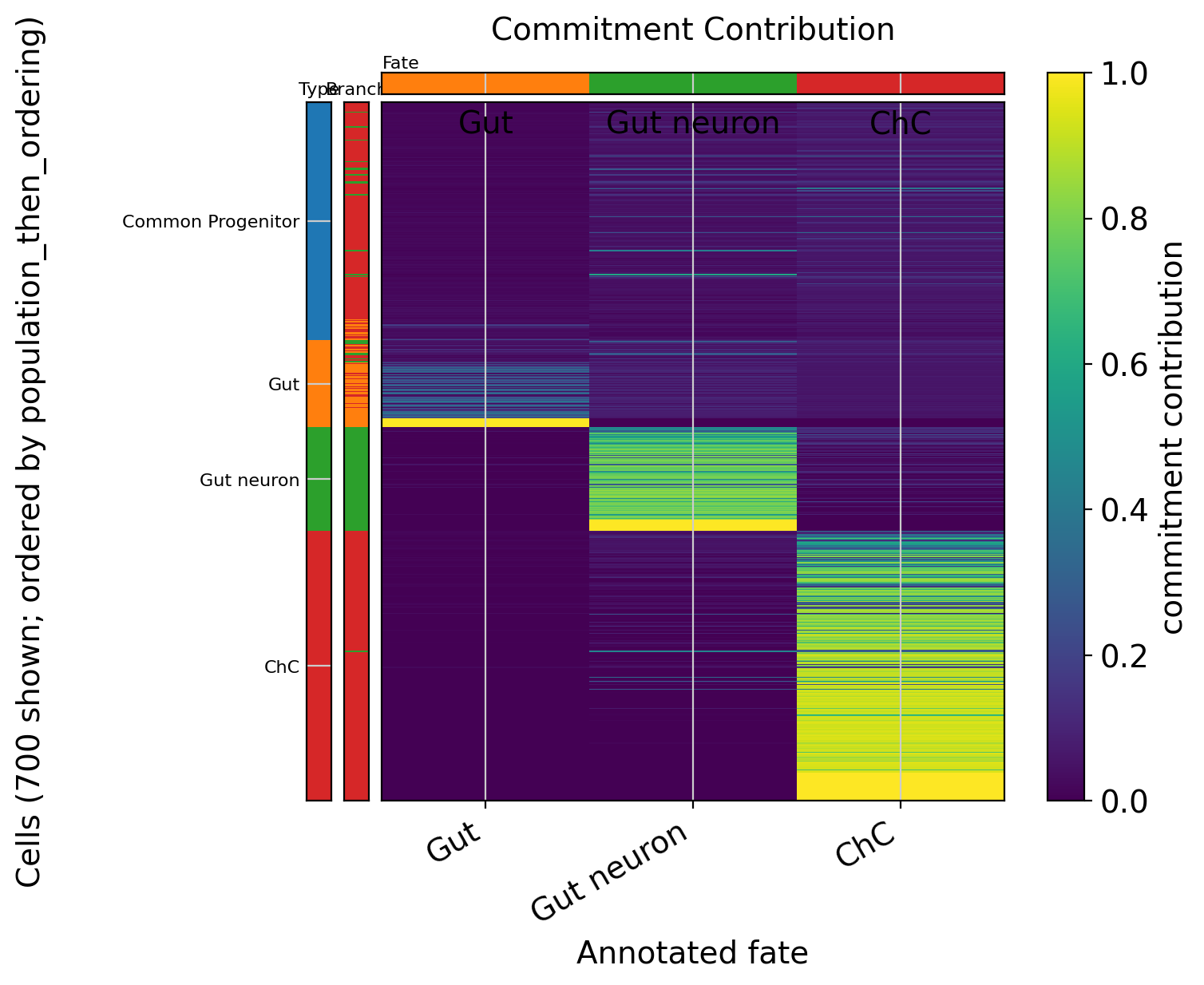
9. Population summaries and the retrograde Gut result
[10]:
selected = adata.obs.loc[result.cell_ids].copy()
selected["future_fate_reach"] = result.future_fate_reach
selected["future_fate_specificity"] = result.future_fate_specificity
selected["reach_supported_specificity"] = result.reach_supported_specificity
selected["signed_progression"] = result.signed_progression
selected["ordering_third"] = ordering_thirds(selected[ORDERING_KEY].to_numpy(float))
for fate_index, fate in enumerate(FATES):
    selected[f"affinity_{fate}"] = result.future_fate_affinity[:, fate_index]

population_summary = selected.groupby("cell_type_new", observed=True).agg(
    n_cells=("future_fate_reach", "size"),
    mean_reach=("future_fate_reach", "mean"),
    mean_specificity=("future_fate_specificity", "mean"),
    mean_supported_specificity=("reach_supported_specificity", "mean"),
    mean_progression=("signed_progression", "mean"),
    forward_fraction=("signed_progression", lambda values: float(np.mean(values > 0))),
)
display(population_summary)
population_summary.to_csv(OUTPUT_DIR / "population_summary.csv")

branch_thirds = (
    selected[selected["cell_type_new"].astype(str).isin(FATES)]
    .groupby(["cell_type_new", "ordering_third"], observed=True)
    .agg(
        n_cells=("future_fate_reach", "size"),
        mean_reach=("future_fate_reach", "mean"),
        mean_specificity=("future_fate_specificity", "mean"),
        mean_progression=("signed_progression", "mean"),
        forward_fraction=("signed_progression", lambda values: float(np.mean(values > 0))),
    )
)
display(branch_thirds)
branch_thirds.to_csv(OUTPUT_DIR / "branch_ordering_thirds.csv")
| n_cells | mean_reach | mean_specificity | mean_supported_specificity | mean_progression | forward_fraction | |
|---|---|---|---|---|---|---|
| cell_type_new | ||||||
| ChC | 762 | 0.807670 | 0.874619 | 0.744100 | 0.039342 | 0.674541 |
| Common Progenitor | 675 | 0.155633 | 0.122960 | 0.024555 | 0.020214 | 0.629630 |
| Gut | 245 | 0.387852 | 0.211938 | 0.149273 | -0.155898 | 0.106122 |
| Gut neuron | 294 | 0.779802 | 0.798632 | 0.639331 | 0.029544 | 0.612245 |
| n_cells | mean_reach | mean_specificity | mean_progression | forward_fraction | ||
|---|---|---|---|---|---|---|
| cell_type_new | ordering_third | |||||
| ChC | early | 168 | 0.595579 | 0.673931 | 0.117944 | 0.928571 |
| late | 315 | 0.935115 | 0.987162 | -0.007118 | 0.476190 | |
| middle | 279 | 0.791490 | 0.868398 | 0.044466 | 0.745520 | |
| Gut | early | 1 | 0.238327 | 0.009248 | 0.111598 | 1.000000 |
| late | 229 | 0.398183 | 0.222419 | -0.162212 | 0.091703 | |
| middle | 15 | 0.240103 | 0.065443 | -0.077343 | 0.266667 | |
| Gut neuron | early | 46 | 0.684211 | 0.545371 | 0.128289 | 0.978261 |
| late | 19 | 1.000000 | 1.000000 | -0.149300 | 0.000000 | |
| middle | 229 | 0.780733 | 0.832798 | 0.024547 | 0.589520 |
10. Population-level composition and pairwise fate balance
[11]:
fig, axes = plt.subplots(1, 3, figsize=(18, 5))
scorer.plot_commitment_bar(result, population="root", metric="commitment_composition", ax=axes[0])
scorer.plot_population_commitment(
    result,
    population="root",
    metric="mean_commitment_contribution",
    ax=axes[1],
)
scorer.plot_pairwise_cs(result, population="root", ax=axes[2])
fig.tight_layout()
fig.savefig(OUTPUT_DIR / "root_population_summaries.png", dpi=200, bbox_inches="tight")
plt.show()
11. Display-only RNA-velocity diagnostics
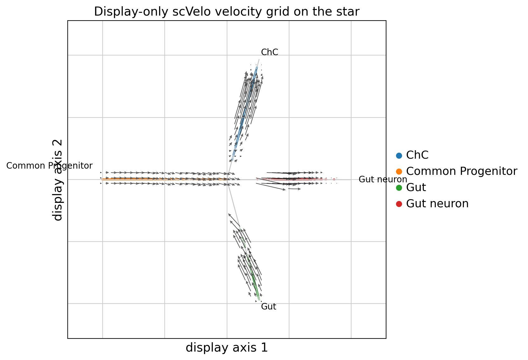
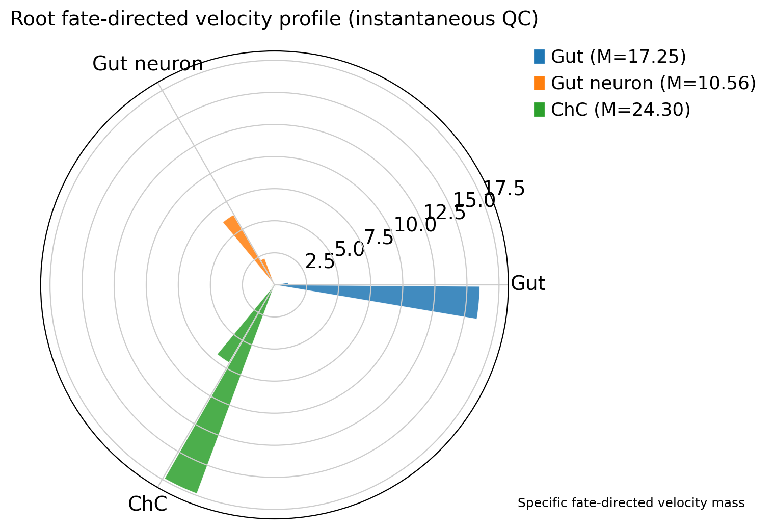
The primary scCS result above is the discounted future-fate model. The figures below are optional RNA-velocity quality-control views. They use a separate instantaneous scorer and therefore do not define future-fate affinity, reach, specificity, or entropy.
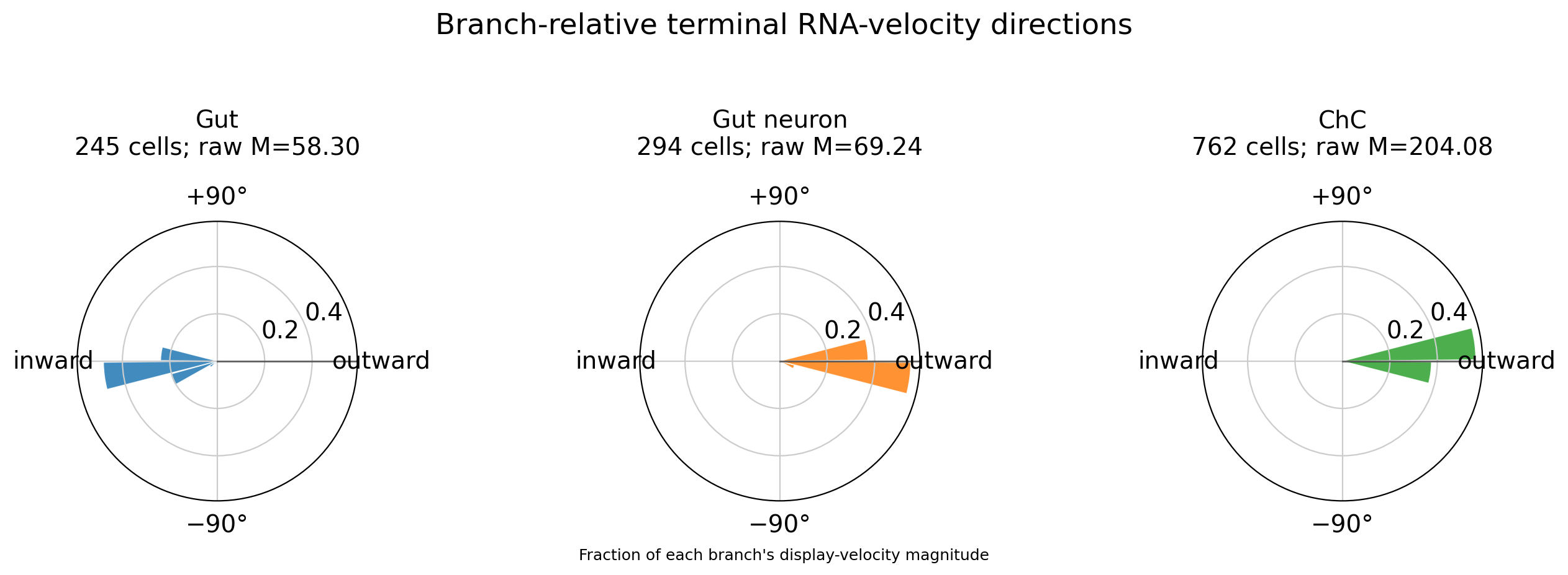
A straight star cannot preserve every turn or loop of the original manifold. We therefore show (1) the native scVelo projection on the star, (2) a root fate-directed rose after removing incoming-root progression, and (3) separate branch-relative roses in which each annotated terminal population retains its identity. In the branch-relative panels, outward is 0°, transverse motion is ±90°, and inward motion is 180°.
[12]:
# First summarize the scientific future-fate result. This table and the root
# future-fate composition plot answer which fate is dominant. Display-space
# arrows answer a different question and can be curved or retrograde.
terminal_labels = np.asarray(result.embedding.selected_labels).astype(str)
terminal_qc_rows = []
for fate_index, fate in enumerate(FATES):
    fate_mask = result.terminal_mask & (terminal_labels == fate)
    terminal_qc_rows.append(
        {
            "fate": fate,
            "n_cells": int(fate_mask.sum()),
            "mean_own_future_fate_affinity": float(
                np.nanmean(result.future_fate_affinity[fate_mask, fate_index])
            ),
            "mean_future_fate_reach": float(np.nanmean(result.future_fate_reach[fate_mask])),
            "mean_signed_progression": float(np.nanmean(result.signed_progression[fate_mask])),
        }
    )
display(pd.DataFrame(terminal_qc_rows).set_index("fate"))

# Build a separate instantaneous scorer only for RNA-velocity display QC.
# This does not alter the primary discounted future-fate result.
instantaneous_display_scorer = scCS.SingleScorer(
    adata,
    root=ROOT,
    branches=FATES,
    obs_key="cell_type_new",
)
instantaneous_display_scorer.build_embedding(
    ordering_metric=ORDERING_KEY,
    write_to_adata=True,
    verbose=False,
)
instantaneous_display_scorer.fit(scoring_mode="instantaneous", verbose=False)
instantaneous_display_result = instantaneous_display_scorer.score(
    write_to_adata=False,
    verbose=False,
)

# Native scVelo projection onto the straightened star. Curved, loop-like, or
# retrograde source trajectories can therefore look inward on some branches.
fig, ax = plt.subplots(figsize=(8, 6))
instantaneous_display_scorer.plot_velocity_embedding_grid(
    instantaneous_display_result,
    population="all",
    density=0.9,
    smooth=0.55,
    min_mass=1.0,
    n_neighbors=50,
    projection_mode="scvelo",
    title="Display-only scVelo velocity grid on the star",
    ax=ax,
)
fig.tight_layout()
fig.savefig(OUTPUT_DIR / "display_velocity_grid.png", dpi=200, bbox_inches="tight")
plt.show()

# Root fate-directed velocity after removing incoming-root progression. This
# is the closest analogue of the familiar binned commitment rose and does not
# assign the incoming root direction to a terminal sector.
root_rose = plt.figure(figsize=(8.5, 6.5))
root_rose_ax = root_rose.add_subplot(111, projection="polar")
instantaneous_display_scorer.plot_rose(
    instantaneous_display_result,
    population="root",
    mode="branch",
    n_bins=36,
    normalization="mass",
    title="Root fate-directed velocity profile (instantaneous QC)",
    ax=root_rose_ax,
)
root_rose.subplots_adjust(right=0.72)
root_rose.savefig(OUTPUT_DIR / "root_branch_velocity_rose.png", dpi=200, bbox_inches="tight")
plt.show()

# Terminal branches are shown separately. Each panel keeps cells attached to
# their annotated branch: 0° is outward, ±90° is transverse, and 180° is
# inward. Thus a retrograde Delta, Epsilon, or Gut vector is never relabeled as
# movement toward a different fate merely because of the 2D star layout.
branch_profiles = instantaneous_display_scorer.plot_branch_velocity_profiles(
    instantaneous_display_result,
    n_bins=24,
    normalization="within_branch",
    projection_mode="scvelo",
    title="Branch-relative terminal RNA-velocity directions",
)
branch_profiles.savefig(
    OUTPUT_DIR / "branch_relative_velocity_profiles.png",
    dpi=200,
    bbox_inches="tight",
)
plt.show()
| n_cells | mean_own_future_fate_affinity | mean_future_fate_reach | mean_signed_progression | |
|---|---|---|---|---|
| fate | ||||
| Gut | 245 | 0.516848 | 0.387852 | -0.155898 |
| Gut neuron | 294 | 0.925179 | 0.779802 | 0.029544 |
| ChC | 762 | 0.951905 | 0.807670 | 0.039342 |
computing velocity embedding
    finished (0:00:00)
computing velocity embedding
    finished (0:00:00)
12. Gene expression on the star
[13]:
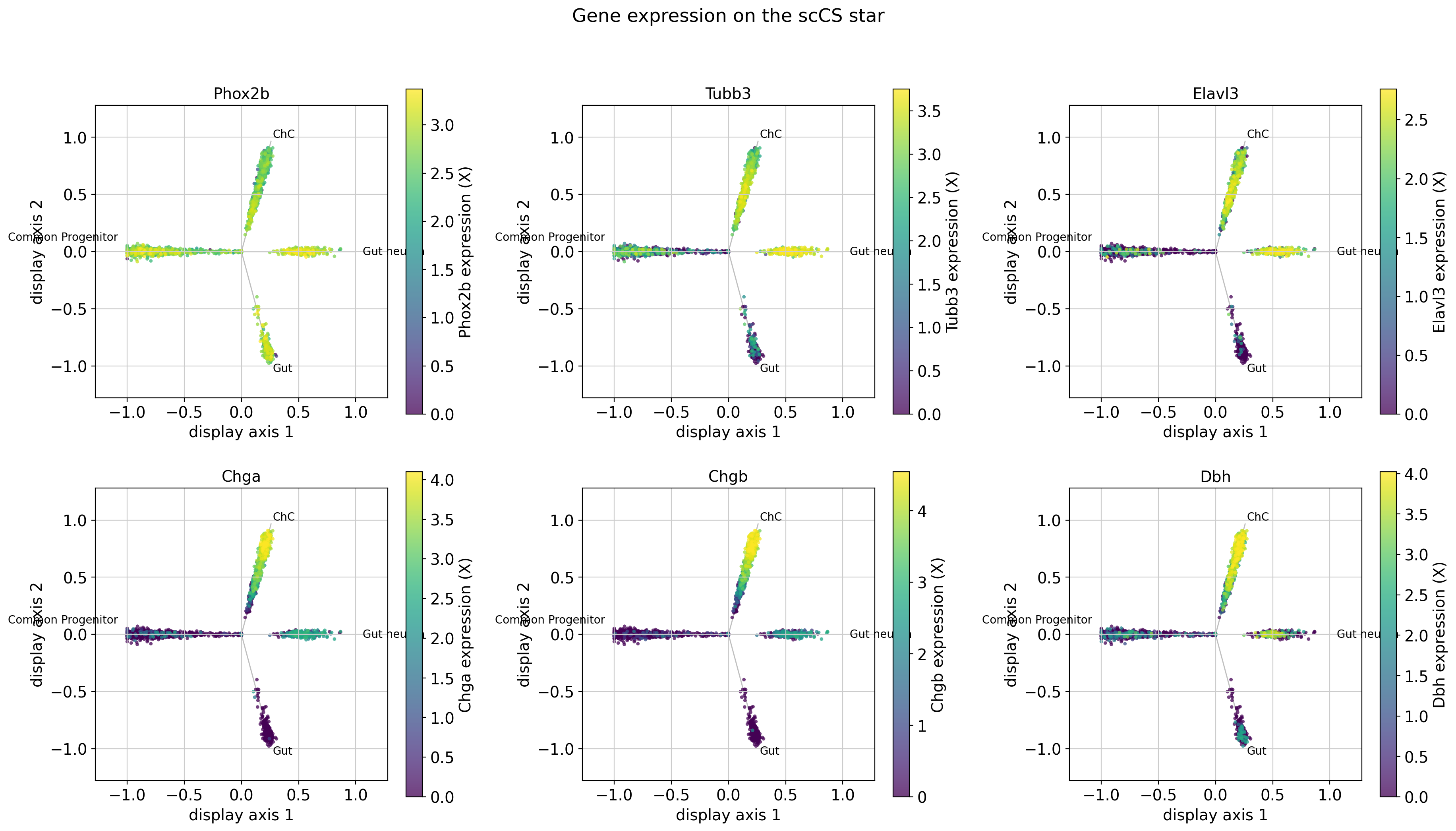
marker_candidates = [
    "Sox10",
    "Foxd3",
    "Phox2b",
    "Tubb3",
    "Elavl3",
    "Chga",
    "Chgb",
    "Th",
    "Dbh",
]
markers, missing_markers = resolve_present_genes(adata, marker_candidates)
print("Resolved markers:", markers)
print("Missing markers:", missing_markers)
if markers:
    marker_fig = scorer.plot_gene_expression_star(
        markers,
        result,
        ncols=3,
        shared_scale=False,
        terminal_layout="ordering",
    )
    marker_fig.savefig(OUTPUT_DIR / "marker_expression_stars.png", dpi=200, bbox_inches="tight")
    plt.show()
Resolved markers: ['Phox2b', 'Tubb3', 'Elavl3', 'Chga', 'Chgb', 'Dbh']
Missing markers: ['Sox10', 'Foxd3', 'Th']
13. Expression trends and exploratory gene associations
[14]:
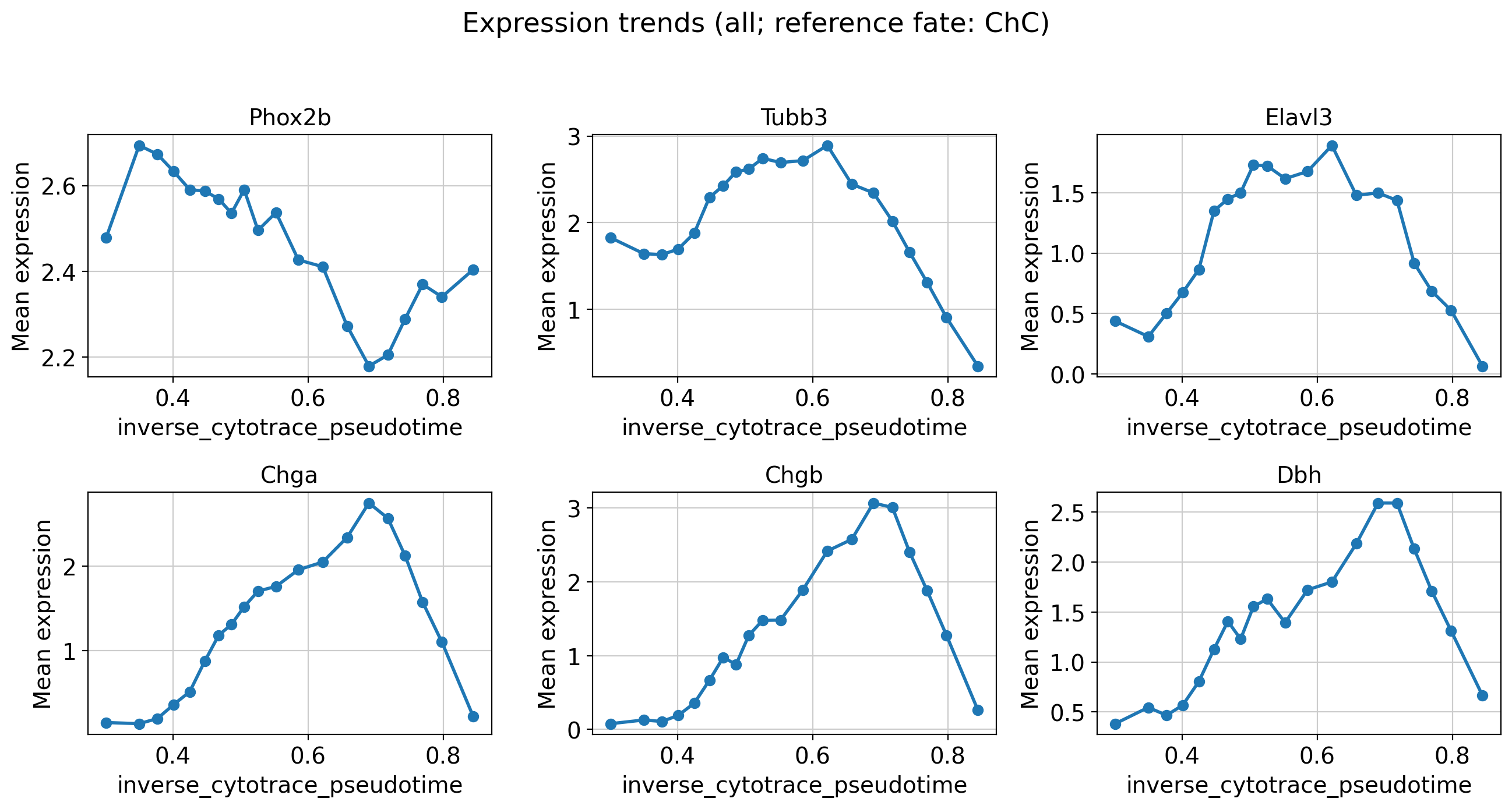
if markers:
    trend_fig = scorer.plot_expression_trends(
        markers,
        result,
        x_axis="ordering",
        population="all",
        n_bins=20,
        ncols=3,
    )
    trend_fig.savefig(OUTPUT_DIR / "marker_expression_trends.png", dpi=200, bbox_inches="tight")
    plt.show()

association = scorer.get_commitment_associated_genes(
    outcome="future_fate_affinity",
    fate_names=FATES,
    population="root",
    inference_unit="cell_exploratory",
    pseudotime_key=ORDERING_KEY,
    min_cells=100,
    min_feature_cells=10,
    min_feature_fraction=0.01,
    n_top_genes=30,
    verbose=True,
)
for fate in FATES:
    print("\n", fate)
    display(association.top(fate, n=15))
association.export(OUTPUT_DIR, prefix="future_fate_gene_association")
[scCS] Candidate commitment-associated genes: Gut
        inference_unit=cell_exploratory; matrix=X; n_units=675; tested_genes=811
 rank    gene   effect   pvalue_adj  significant
    1  Col5a1 0.485261 3.373593e-38         True
    2   Lama4 0.459167 7.590007e-34         True
    3   Hspg2 0.438345 1.377937e-30         True
    4    Mcam 0.433175 6.778292e-30         True
    5   Lamb1 0.410938 1.230403e-26         True
    6 Col18a1 0.372944 1.160676e-21         True
    7  Tagln2 0.369894 2.515631e-21         True
    8   Sparc 0.357539 5.845513e-20         True
    9  Sorbs1 0.337323 1.150607e-17         True
   10  Camk2b 0.332076 3.902908e-17         True
   11   Postn 0.332067 3.902908e-17         True
   12   Wwtr1 0.328782 8.119904e-17         True
   13 Micall1 0.328721 8.119904e-17         True
   14    Ngfr 0.322114 3.959277e-16         True
   15   Lamc1 0.314530 2.240800e-15         True
   16    Utrn 0.308363 9.123179e-15         True
   17  Col4a2 0.308078 9.342270e-15         True
   18   Spon1 0.300278 5.328067e-14         True
   19  Col4a1 0.300102 5.329232e-14         True
   20    Irs1 0.288721 6.046698e-13         True
   21    Mest 0.287541 7.519048e-13         True
   22    Nid1 0.286447 9.170804e-13         True
   23    Sox8 0.280049 3.306476e-12         True
   24   Megf6 0.275438 8.279653e-12         True
   25  Rhbdf1 0.275248 8.352061e-12         True
   26    Lrp1 0.273525 1.151089e-11         True
   27  Akap12 0.272943 1.237408e-11         True
   28    Lmna 0.272891 1.237408e-11         True
   29 Col16a1 0.272469 1.311865e-11         True
   30  Tcirg1 0.267583 3.334933e-11         True

[scCS] Candidate commitment-associated genes: Gut neuron
        inference_unit=cell_exploratory; matrix=X; n_units=675; tested_genes=811
 rank     gene   effect   pvalue_adj  significant
    1   Chrnb4 0.363621 1.717270e-20         True
    2    Celf2 0.309912 4.876724e-15         True
    3 Serpini1 0.296371 8.386112e-14         True
    4     Rbp1 0.291200 2.477431e-13         True
    5     Dll1 0.285390 7.663913e-13         True
    6      Cd9 0.272488 1.056612e-11         True
    7   Phox2b 0.257167 1.699414e-10         True
    8  Slc18a2 0.251240 4.958618e-10         True
    9    Ednrb 0.245161 1.359559e-09         True
   10     Eya1 0.239936 3.107756e-09         True
   11      Ret 0.232481 1.034079e-08         True
   12   Tmsb4x 0.230940 1.324405e-08         True
   13    Fgf13 0.226635 2.464155e-08         True
   14    Srrm4 0.218251 8.841821e-08         True
   15    Dhrs3 0.216010 1.207640e-07         True
   16   Elavl4 0.179148 1.591619e-05         True
   17      Gal 0.166248 7.015918e-05         True
   18  Fam163a 0.161599 1.182988e-04         True
   19    Ltbp1 0.157941 1.688875e-04         True
   20  Gadd45g 0.157854 1.696503e-04         True
   21    Ddah1 0.156555 1.918314e-04         True
   22     Scg5 0.141439 8.671057e-04         True
   23  Fam184b 0.140249 9.665274e-04         True
   24      Cpe 0.140187 9.682715e-04         True
   25  Slitrk6 0.139705 1.012530e-03         True
   26   Tmeff2 0.136944 1.309116e-03         True
   27  Slc29a4 0.131577 2.072815e-03         True
   28    Ube2c 0.130522 2.266135e-03         True
   29     Hes6 0.126707 3.123755e-03         True
   30    Nedd9 0.123953 3.942967e-03         True

[scCS] Candidate commitment-associated genes: ChC
        inference_unit=cell_exploratory; matrix=X; n_units=675; tested_genes=811
 rank     gene   effect   pvalue_adj  significant
    1    Gata3 0.320293 6.171498e-15         True
    2    Tbx20 0.265919 4.297022e-10         True
    3    Htr3a 0.265101 4.297022e-10         True
    4   Cdkn1c 0.253558 2.520190e-09         True
    5   Tfap2b 0.225580 2.578904e-07         True
    6     Pls3 0.206909 3.957827e-06         True
    7    Zdbf2 0.206474 3.957827e-06         True
    8   Adam23 0.203170 5.997808e-06         True
    9    Scrg1 0.200918 7.780744e-06         True
   10    Padi2 0.194298 1.582217e-05         True
   11   Crabp2 0.188008 3.414284e-05         True
   12    Myo5b 0.186276 3.997004e-05         True
   13   Tfap2a 0.177556 1.056930e-04         True
   14    Stra6 0.170624 2.276990e-04         True
   15    Htr3b 0.170271 2.301797e-04         True
   16      Ddc 0.169418 2.476214e-04         True
   17     Cst3 0.162114 4.883255e-04         True
   18    Peg10 0.156921 8.075719e-04         True
   19 Arhgap19 0.155633 9.133913e-04         True
   20 Ndufa4l2 0.154709 9.488460e-04         True
   21     Tlx2 0.154522 9.488460e-04         True
   22     Dlk1 0.152103 1.216934e-03         True
   23    Cdh11 0.151127 1.319936e-03         True
   24    Tppp3 0.149060 1.570026e-03         True
   25    Luzp2 0.144737 2.318172e-03         True
   26      Kit 0.144215 2.406859e-03         True
   27    Tnnt3 0.143386 2.581147e-03         True
   28    Mfap4 0.139096 3.762434e-03         True
   29     Cdh6 0.132523 6.732329e-03         True
   30     Meg3 0.132477 6.732329e-03         True

 Gut
| gene | effect | pvalue | pvalue_adj | feature_mean | feature_sd | n_detected_cells | n_units | significant | absolute_effect | rank | |
|---|---|---|---|---|---|---|---|---|---|---|---|
| 0 | Col5a1 | 0.485261 | 4.159794e-41 | 3.373593e-38 | 1.964407 | 0.947295 | 579 | 675 | True | 0.485261 | 1 |
| 1 | Lama4 | 0.459167 | 1.871765e-36 | 7.590007e-34 | 1.773734 | 1.000479 | 544 | 675 | True | 0.459167 | 2 |
| 2 | Hspg2 | 0.438345 | 5.097178e-33 | 1.377937e-30 | 0.918172 | 0.899727 | 378 | 675 | True | 0.438345 | 3 |
| 3 | Mcam | 0.433175 | 3.343177e-32 | 6.778292e-30 | 2.143249 | 0.945579 | 590 | 675 | True | 0.433175 | 4 |
| 4 | Lamb1 | 0.410938 | 7.585717e-29 | 1.230403e-26 | 1.813068 | 0.940148 | 563 | 675 | True | 0.410938 | 5 |
| 5 | Col18a1 | 0.372944 | 1.144933e-23 | 1.160676e-21 | 1.921003 | 0.971373 | 572 | 675 | True | 0.372944 | 6 |
| 6 | Tagln2 | 0.369894 | 2.791699e-23 | 2.515631e-21 | 2.127654 | 1.016963 | 574 | 675 | True | 0.369894 | 7 |
| 7 | Sparc | 0.357539 | 9.370120e-22 | 5.845513e-20 | 2.890668 | 0.471350 | 668 | 675 | True | 0.357539 | 8 |
| 8 | Sorbs1 | 0.337323 | 2.128126e-19 | 1.150607e-17 | 1.455308 | 1.035056 | 482 | 675 | True | 0.337323 | 9 |
| 9 | Camk2b | 0.332076 | 8.163270e-19 | 3.902908e-17 | 1.493340 | 0.928660 | 524 | 675 | True | 0.332076 | 10 |
| 10 | Postn | 0.332067 | 8.181189e-19 | 3.902908e-17 | 1.918151 | 1.211993 | 512 | 675 | True | 0.332067 | 11 |
| 11 | Wwtr1 | 0.328782 | 1.873632e-18 | 8.119904e-17 | 2.216385 | 0.644893 | 647 | 675 | True | 0.328782 | 12 |
| 12 | Micall1 | 0.328721 | 1.902320e-18 | 8.119904e-17 | 1.369096 | 1.200335 | 406 | 675 | True | 0.328721 | 13 |
| 13 | Ngfr | 0.322114 | 9.763938e-18 | 3.959277e-16 | 2.010714 | 1.003868 | 566 | 675 | True | 0.322114 | 14 |
| 14 | Lamc1 | 0.314530 | 6.078618e-17 | 2.240800e-15 | 1.610098 | 0.936293 | 541 | 675 | True | 0.314530 | 15 |
Gut neuron
| gene | effect | pvalue | pvalue_adj | feature_mean | feature_sd | n_detected_cells | n_units | significant | absolute_effect | rank | |
|---|---|---|---|---|---|---|---|---|---|---|---|
| 0 | Chrnb4 | 0.363621 | 1.693978e-22 | 1.717270e-20 | 0.884235 | 1.126394 | 282 | 675 | True | 0.363621 | 1 |
| 1 | Celf2 | 0.309912 | 1.803967e-16 | 4.876724e-15 | 2.413041 | 0.481743 | 664 | 675 | True | 0.309912 | 2 |
| 2 | Serpini1 | 0.296371 | 3.929374e-15 | 8.386112e-14 | 1.026285 | 1.147788 | 323 | 675 | True | 0.296371 | 3 |
| 3 | Rbp1 | 0.291200 | 1.221914e-14 | 2.477431e-13 | 3.046686 | 0.412748 | 673 | 675 | True | 0.291200 | 4 |
| 4 | Dll1 | 0.285390 | 4.252479e-14 | 7.663913e-13 | 0.642346 | 1.004160 | 214 | 675 | True | 0.285390 | 5 |
| 5 | Cd9 | 0.272488 | 6.123400e-13 | 1.056612e-11 | 2.153465 | 0.689199 | 631 | 675 | True | 0.272488 | 6 |
| 6 | Phox2b | 0.257167 | 1.215364e-11 | 1.699414e-10 | 2.511418 | 0.507439 | 666 | 675 | True | 0.257167 | 7 |
| 7 | Slc18a2 | 0.251240 | 3.668521e-11 | 4.958618e-10 | 1.369748 | 1.047893 | 460 | 675 | True | 0.251240 | 8 |
| 8 | Ednrb | 0.245161 | 1.106423e-10 | 1.359559e-09 | 3.201430 | 0.363540 | 675 | 675 | True | 0.245161 | 9 |
| 9 | Eya1 | 0.239936 | 2.791368e-10 | 3.107756e-09 | 1.019634 | 0.999943 | 379 | 675 | True | 0.239936 | 10 |
| 10 | Ret | 0.232481 | 1.007303e-09 | 1.034079e-08 | 2.427413 | 1.007805 | 602 | 675 | True | 0.232481 | 11 |
| 11 | Tmsb4x | 0.230940 | 1.306442e-09 | 1.324405e-08 | 2.849985 | 0.377604 | 668 | 675 | True | 0.230940 | 12 |
| 12 | Fgf13 | 0.226635 | 2.673806e-09 | 2.464155e-08 | 1.338304 | 1.064584 | 444 | 675 | True | 0.226635 | 13 |
| 13 | Srrm4 | 0.218251 | 1.035725e-08 | 8.841821e-08 | 0.394998 | 0.763041 | 160 | 675 | True | 0.218251 | 14 |
| 14 | Dhrs3 | 0.216010 | 1.474185e-08 | 1.207640e-07 | 1.299431 | 1.185342 | 397 | 675 | True | 0.216010 | 15 |
ChC
| gene | effect | pvalue | pvalue_adj | feature_mean | feature_sd | n_detected_cells | n_units | significant | absolute_effect | rank | |
|---|---|---|---|---|---|---|---|---|---|---|---|
| 0 | Gata3 | 0.320293 | 1.521948e-17 | 6.171498e-15 | 0.256525 | 0.683459 | 95 | 675 | True | 0.320293 | 1 |
| 1 | Tbx20 | 0.265919 | 2.257416e-12 | 4.297022e-10 | 0.157420 | 0.546793 | 60 | 675 | True | 0.265919 | 2 |
| 2 | Htr3a | 0.265101 | 2.649212e-12 | 4.297022e-10 | 0.220528 | 0.710026 | 66 | 675 | True | 0.265101 | 3 |
| 3 | Cdkn1c | 0.253558 | 2.389436e-11 | 2.520190e-09 | 2.755475 | 0.681492 | 668 | 675 | True | 0.253558 | 4 |
| 4 | Tfap2b | 0.225580 | 3.179907e-09 | 2.578904e-07 | 0.435354 | 0.732454 | 198 | 675 | True | 0.225580 | 5 |
| 5 | Pls3 | 0.206909 | 5.944413e-08 | 3.957827e-06 | 2.281151 | 0.961091 | 596 | 675 | True | 0.206909 | 6 |
| 6 | Zdbf2 | 0.206474 | 6.344236e-08 | 3.957827e-06 | 0.520088 | 0.832358 | 208 | 675 | True | 0.206474 | 7 |
| 7 | Adam23 | 0.203170 | 1.035380e-07 | 5.997808e-06 | 0.961757 | 0.977666 | 372 | 675 | True | 0.203170 | 8 |
| 8 | Scrg1 | 0.200918 | 1.439102e-07 | 7.780744e-06 | 0.359461 | 0.726299 | 142 | 675 | True | 0.200918 | 9 |
| 9 | Padi2 | 0.194298 | 3.706797e-07 | 1.582217e-05 | 0.652577 | 0.964456 | 229 | 675 | True | 0.194298 | 10 |
| 10 | Crabp2 | 0.188008 | 8.840934e-07 | 3.414284e-05 | 0.457361 | 0.799198 | 182 | 675 | True | 0.188008 | 11 |
| 11 | Myo5b | 0.186276 | 1.117582e-06 | 3.997004e-05 | 0.160684 | 0.535615 | 60 | 675 | True | 0.186276 | 12 |
| 12 | Tfap2a | 0.177556 | 3.518755e-06 | 1.056930e-04 | 0.539686 | 0.682610 | 299 | 675 | True | 0.177556 | 13 |
| 13 | Stra6 | 0.170624 | 8.422899e-06 | 2.276990e-04 | 0.299689 | 0.709857 | 112 | 675 | True | 0.170624 | 14 |
| 14 | Htr3b | 0.170271 | 8.798483e-06 | 2.301797e-04 | 0.062199 | 0.343268 | 25 | 675 | True | 0.170271 | 15 |
[14]:
['tutorial_outputs/schwann_single/future_fate_gene_association_Gut.csv',
 'tutorial_outputs/schwann_single/future_fate_gene_association_Gut_neuron.csv',
 'tutorial_outputs/schwann_single/future_fate_gene_association_ChC.csv',
 'tutorial_outputs/schwann_single/future_fate_gene_association_metadata.json']
14. Optional replicate-aware gene association
The RegVelo object may contain plate or sample metadata. A plate-level analysis is only appropriate when the units are sufficiently numerous and scientifically defensible; plate can be confounded with developmental time. The code below runs only when a usable key is present.
[15]:
replicate_candidates = [key for key in ("plate", "sample", "sample_id") if key in adata.obs]
if replicate_candidates:
    replicate_key = replicate_candidates[0]
    root_units = adata.obs.loc[result.cell_ids[result.root_mask], replicate_key].astype(str)
    unit_counts = root_units.value_counts()
    eligible = unit_counts[unit_counts >= 5]
    print("Candidate replicate key:", replicate_key)
    display(unit_counts.to_frame("root_cells"))
    if len(eligible) >= 6:
        replicate_association = scorer.get_commitment_associated_genes(
            outcome="future_fate_affinity",
            fate_names=FATES,
            population="root",
            inference_unit="replicate",
            replicate_key=replicate_key,
            pseudotime_key=None,
            min_replicates=6,
            min_cells_per_replicate=5,
            min_feature_cells=5,
            verbose=True,
        )
        replicate_association.export(
            OUTPUT_DIR,
            prefix="replicate_future_fate_gene_association",
        )
    else:
        print("Too few eligible units for replicate-level association.")
else:
    print("No plausible replicate column found; section skipped.")
No plausible replicate column found; section skipped.
15. Horizon and anchor sensitivity
[16]:
sensitivity = {}
for horizon in (32, 64, 128):
    for quantile in (0.85, 0.90, 0.95):
        scorer.fit(
            scoring_mode="future_fate",
            future_fate_options={
                **FUTURE_OPTIONS,
                "effective_horizon": horizon,
                "anchor_quantile": quantile,
                "verbose": False,
            },
            verbose=False,
        )
        sensitivity[(horizon, quantile)] = scorer.score(
            write_to_adata=False,
            verbose=False,
        )
primary = sensitivity[(64, 0.90)]
root = primary.root_mask
sensitivity_table = pd.DataFrame(
    {
        "criterion": [
            "median root affinity JS: h64 vs h128",
            "median root affinity JS: q0.85 vs q0.95",
            "mean root reach: h32",
            "mean root reach: h64",
            "mean root reach: h128",
        ],
        "value": [
            np.nanmedian(
                row_js(
                    sensitivity[(64, 0.90)].future_fate_affinity[root],
                    sensitivity[(128, 0.90)].future_fate_affinity[root],
                )
            ),
            np.nanmedian(
                row_js(
                    sensitivity[(64, 0.85)].future_fate_affinity[root],
                    sensitivity[(64, 0.95)].future_fate_affinity[root],
                )
            ),
            sensitivity[(32, 0.90)].future_fate_reach[root].mean(),
            sensitivity[(64, 0.90)].future_fate_reach[root].mean(),
            sensitivity[(128, 0.90)].future_fate_reach[root].mean(),
        ],
    }
)
display(sensitivity_table)
sensitivity_table.to_csv(OUTPUT_DIR / "sensitivity_summary.csv", index=False)
result = primary
| criterion | value | |
|---|---|---|
| 0 | median root affinity JS: h64 vs h128 | 0.000612 |
| 1 | median root affinity JS: q0.85 vs q0.95 | 0.010306 |
| 2 | mean root reach: h32 | 0.106764 |
| 3 | mean root reach: h64 | 0.155633 |
| 4 | mean root reach: h128 | 0.211841 |
16. Optional deterministic sensitivity
The main Schwann analysis uses the dynamical model. This optional section fits a second, deterministic model from the original RegVelo object and compares the continuous root-cell outputs. It is a robustness analysis, not an alternative default.
[17]:
RUN_DETERMINISTIC_SENSITIVITY = False

if RUN_DETERMINISTIC_SENSITIVITY:
    # Refit a fresh deterministic model only when a cross-model comparison is
    # scientifically useful. The primary tutorial result remains dynamical.
    adata_deterministic = rgv.datasets.schwann()
    adata_deterministic.var_names_make_unique()
    prepare_schwann_annotations(adata_deterministic)
    ensure_pca_neighbors_moments(
        adata_deterministic,
        n_pcs=30,
        n_neighbors=30,
        preserve_existing_neighbors=True,
    )
    clear_velocity_outputs(adata_deterministic, clear_dynamics=False)
    scv.tl.velocity(
        adata_deterministic,
        mode="deterministic",
        fit_offset=False,
    )
    scv.tl.velocity_graph(adata_deterministic, n_jobs=N_JOBS)
    prepare_schwann_annotations(adata_deterministic)

    scorer_deterministic = scCS.SingleScorer(
        adata_deterministic,
        root=ROOT,
        branches=FATES,
        obs_key="cell_type_new",
    )
    scorer_deterministic.build_embedding(
        ordering_metric=ORDERING_KEY,
        verbose=False,
    )
    scorer_deterministic.fit(
        scoring_mode="future_fate",
        future_fate_options=FUTURE_OPTIONS,
        verbose=False,
    )
    result_deterministic = scorer_deterministic.score(
        write_to_adata=False,
        verbose=False,
    )

    common = pd.Index(result.cell_ids).intersection(result_deterministic.cell_ids)
    dynamical_index = pd.Index(result.cell_ids).get_indexer(common)
    deterministic_index = pd.Index(result_deterministic.cell_ids).get_indexer(common)
    root_common = (
        result.root_mask[dynamical_index] & result_deterministic.root_mask[deterministic_index]
    )

    comparison = pd.Series(
        {
            "mean_root_affinity_JS": np.nanmean(
                row_js(
                    result.future_fate_affinity[dynamical_index][root_common],
                    result_deterministic.future_fate_affinity[deterministic_index][root_common],
                )
            ),
            "signed_progression_rho": spearmanr(
                result.signed_progression[dynamical_index][root_common],
                result_deterministic.signed_progression[deterministic_index][root_common],
            ).statistic,
            "specificity_rho": spearmanr(
                result.future_fate_specificity[dynamical_index][root_common],
                result_deterministic.future_fate_specificity[deterministic_index][root_common],
            ).statistic,
        }
    )
    display(comparison.to_frame("value"))
else:
    print(
        "Set RUN_DETERMINISTIC_SENSITIVITY=True only when a second velocity "
        "model is needed for robustness analysis."
    )
Set RUN_DETERMINISTIC_SENSITIVITY=True only when a second velocity model is needed for robustness analysis.
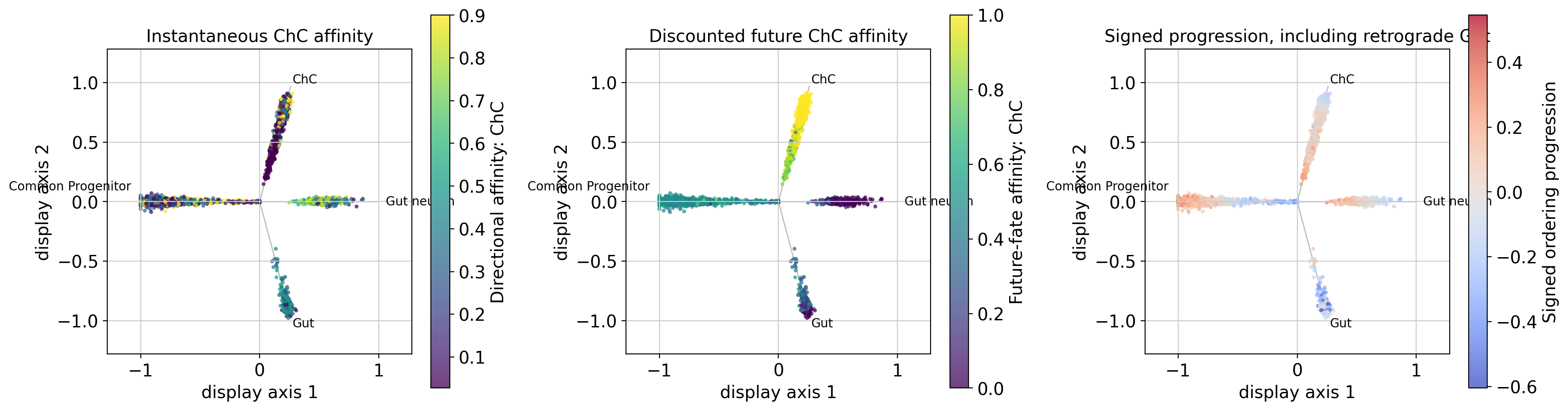
17. Compare future-fate and instantaneous scoring
[18]:
instantaneous = instantaneous_display_result
fig, axes = plt.subplots(1, 3, figsize=(18, 5))
instantaneous_display_scorer.plot_star(
    instantaneous,
    color_by="affinity:ChC",
    title="Instantaneous ChC affinity",
    ax=axes[0],
)
scorer.plot_star(
    result,
    color_by="future_fate_affinity:ChC",
    title="Discounted future ChC affinity",
    ax=axes[1],
)
scorer.plot_star(
    result,
    color_by="signed_progression",
    title="Signed progression, including retrograde Gut",
    cmap="coolwarm",
    ax=axes[2],
)
fig.tight_layout()
fig.savefig(OUTPUT_DIR / "instantaneous_vs_future_fate.png", dpi=200, bbox_inches="tight")
plt.show()
18. Export reproducible analysis objects
[19]:
result.write_to_adata(adata)
adata.write_h5ad(OUTPUT_DIR / f"schwann_{VELOCITY_MODEL}_sccs_future_fate.h5ad")
cell_table = adata.obs.loc[result.cell_ids].copy()
cell_table["future_fate_reach"] = result.future_fate_reach
cell_table["future_fate_specificity"] = result.future_fate_specificity
cell_table["reach_supported_specificity"] = result.reach_supported_specificity
cell_table["signed_progression"] = result.signed_progression
cell_table["unresolved_probability"] = result.unresolved_probability
for fate_index, fate in enumerate(FATES):
    cell_table[f"future_fate_affinity_{fate}"] = result.future_fate_affinity[:, fate_index]
    cell_table[f"future_fate_contribution_{fate}"] = result.future_fate_contribution[:, fate_index]
cell_table.to_csv(OUTPUT_DIR / "cell_level_future_fate_scores.csv")
print("Saved outputs to", OUTPUT_DIR.resolve())
Saved outputs to /home/emil/notebooks/08-tutorials/tutorial_outputs/schwann_single
19. Interpretation checklist
Inverse CytoTRACE is benchmark-specific, not a universal ordering recommendation.
Gut retrograde progression is reported, not corrected away.
Gut identity and Gut progression are separate questions.
Root cells are generally low-specificity; hard dominant-fate labels should be restricted to sufficiently informative cells.
Plate-level candidate-gene analyses require strong caveats about confounding.