Pancreas SingleScorer tutorial¶

This notebook is a complete guide to one supervised pancreas analysis. It starts with the original scVelo manifold and finishes with interpretable scCS outputs, downstream biological context, sensitivity analysis, and reproducible export.

The scientific quantities are kept separate throughout:

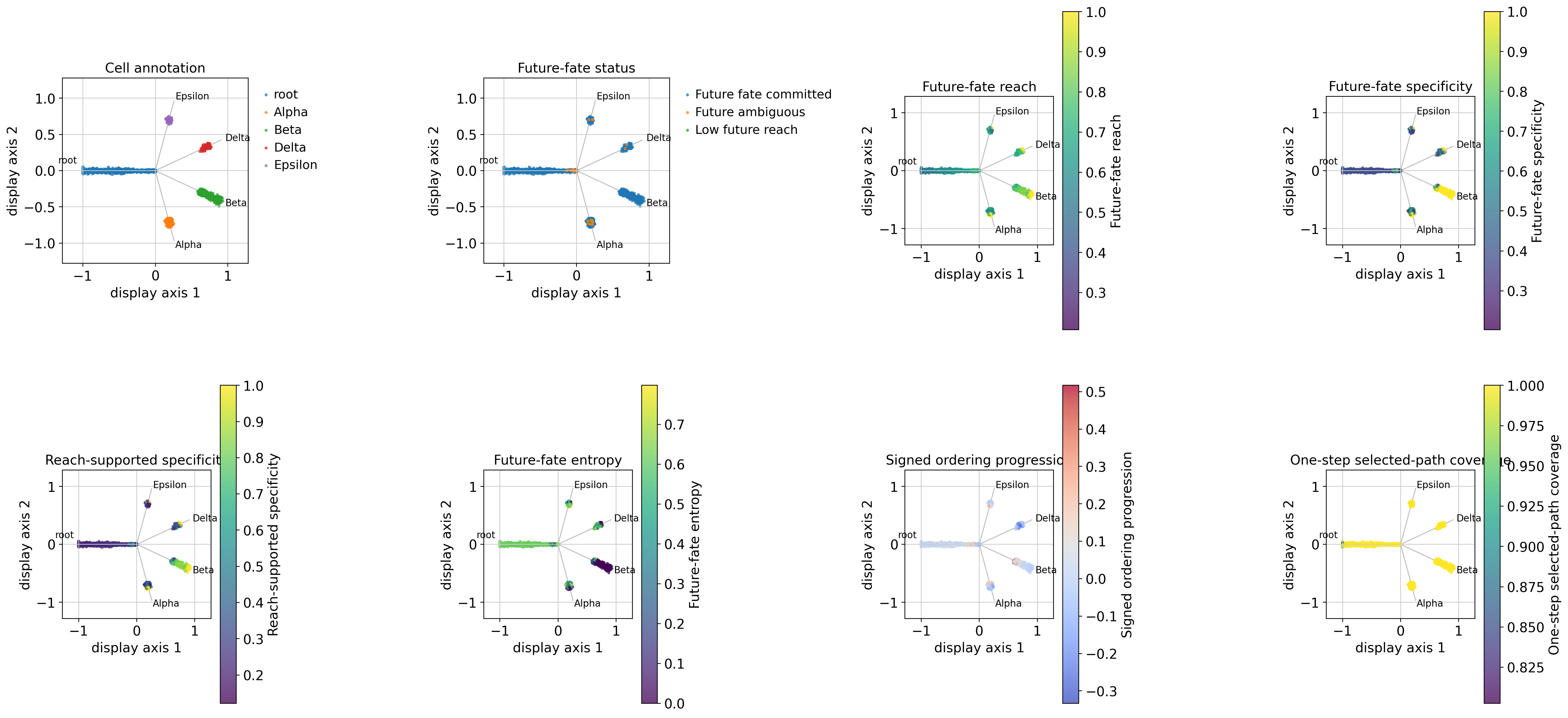
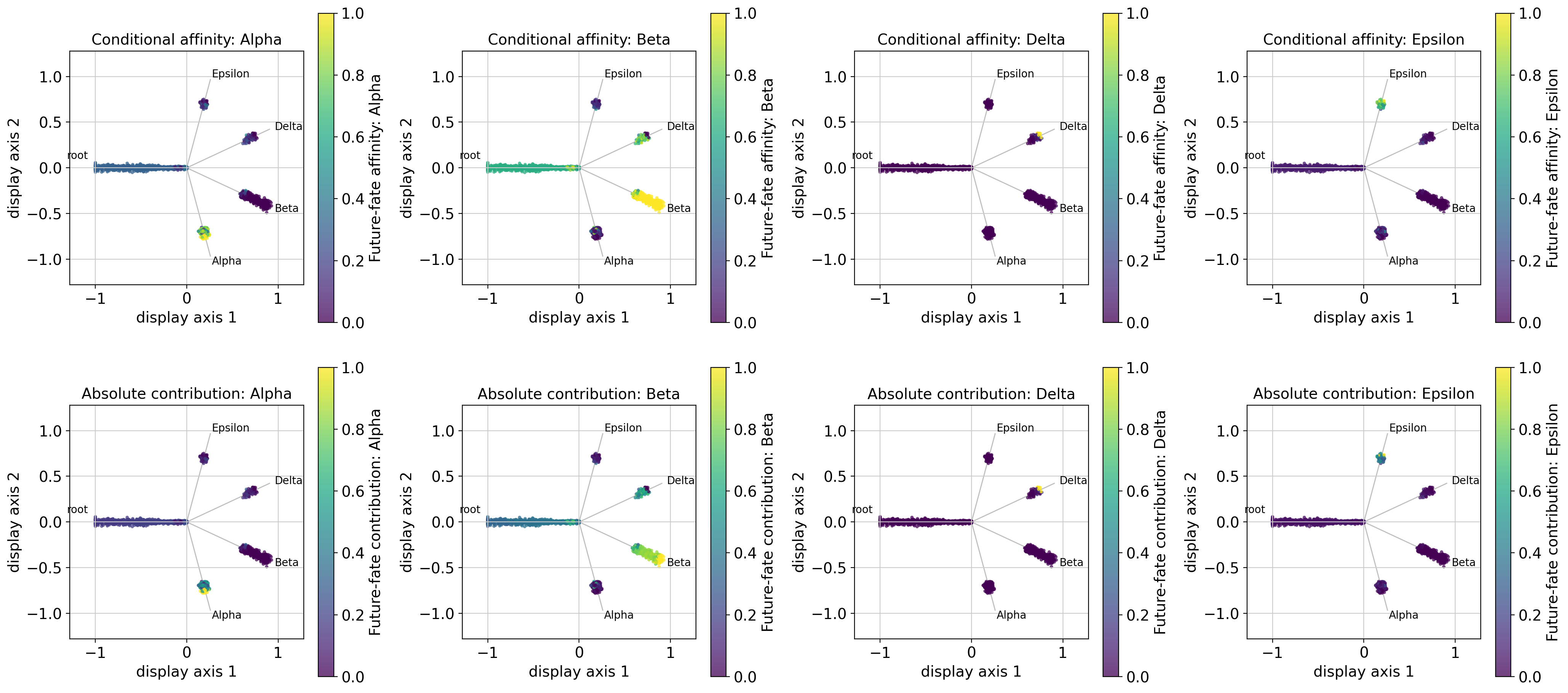
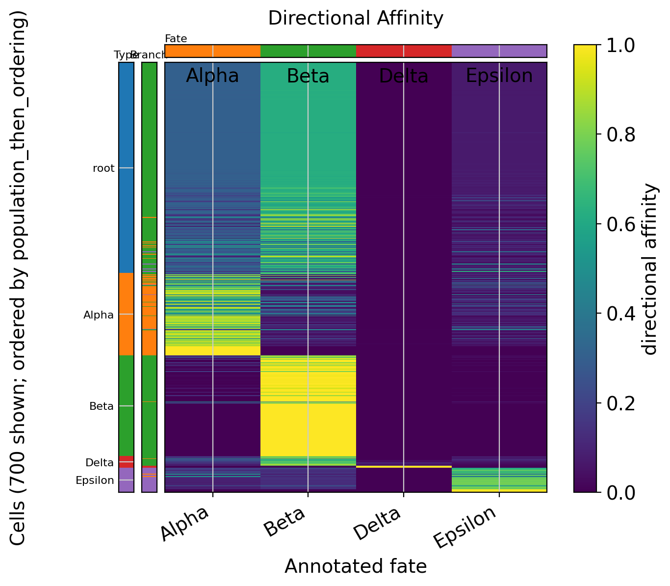
future-fate affinity: conditional identity among the supplied fates;
future-fate reach: discounted probability of reaching a supplied endpoint;
future-fate specificity: decisiveness among the supplied fates;
reach-supported specificity: fate decisiveness weighted by reach;
signed progression: forward, retrograde, or mixed movement along the supplied ordering.

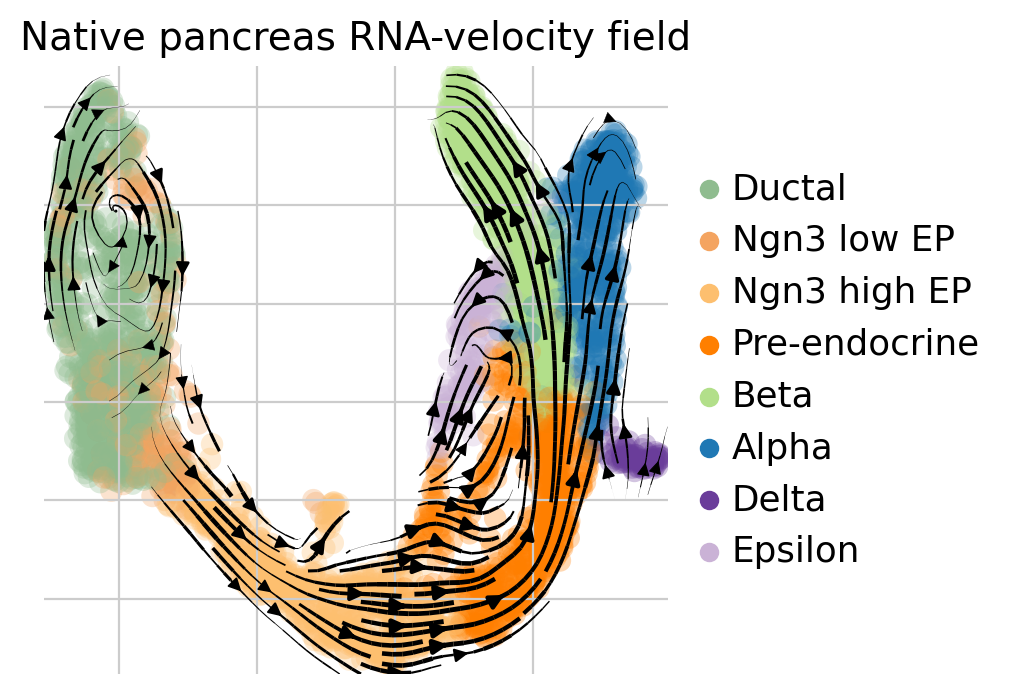
Alpha, Delta, and Epsilon are not required to form simple monotonic rays. Their unusual native velocity patterns are biological results to interpret, not errors that scCS should erase.

Execution provenance. The displayed outputs were generated with scCS 0.8.0.dev33. Version 0.8.0.dev34 changes documentation and tutorial explanation only; the scientific calculations are unchanged.

1. Installation, versions, and reproducibility¶

[1]:

from __future__ import annotations
import warnings

from pathlib import Path
import importlib.metadata as importlib_metadata
import platform
import sys

import matplotlib.pyplot as plt
import numpy as np
import pandas as pd
import scanpy as sc
import scvelo as scv
from scipy.spatial.distance import jensenshannon

import scCS

SEED = 20260714
N_JOBS = 1
sc.settings.verbosity = 2
scv.settings.verbosity = 2
sc.set_figure_params(dpi=100, facecolor="white")

print("Python", sys.version.split()[0])
print("Platform", platform.platform())
print("scCS", scCS.__version__)
print("Scanpy", importlib_metadata.version("scanpy"))
print("scVelo", scv.__version__)

OUTPUT_DIR = Path("tutorial_outputs/pancreas_single")
OUTPUT_DIR.mkdir(parents=True, exist_ok=True)

# Hide known warnings emitted by optional upstream dependencies. These do not
# change the scCS calculation and would otherwise distract from the tutorial.
warnings.filterwarnings(
    "ignore",
    message=r"This process .* is multi-threaded, use of fork\(\) may lead to deadlocks.*",
    category=DeprecationWarning,
)
warnings.filterwarnings(
    "ignore",
    category=DeprecationWarning,
    module=r"cellrank\..*",
)

Python 3.12.13
Platform Linux-6.6.114.1-microsoft-standard-WSL2-x86_64-with-glibc2.39
scCS 0.8.0.dev33
Scanpy 1.11.5
scVelo 0.3.4

2. Load pancreas and fit dynamical RNA velocity¶

Neighbors, moments, kinetic fitting, velocity, and the velocity graph are computed in the original PCA/expression manifold. The supervised star is not used to create neighborhoods or refit velocity.

This tutorial deliberately starts from the public dataset and recomputes the velocity model. No pre-existing scCS cache is assumed. Dynamical fitting can take several minutes, but showing the complete preparation makes every analysis step reproducible for a first-time user.

[2]:

def clear_velocity_outputs(adata, *, clear_dynamics=False):
    """Remove stale velocity fields before fitting a requested model."""
    for key in ("velocity", "velocity_u", "velocity_variance"):
        adata.layers.pop(key, None)
    for key in ("velocity_graph", "velocity_graph_neg", "velocity_params"):
        adata.uns.pop(key, None)
    for key in (
        "velocity_self_transition",
        "root_cells",
        "end_points",
        "velocity_pseudotime",
        "latent_time",
    ):
        if key in adata.obs:
            del adata.obs[key]
    if clear_dynamics:
        for key in list(adata.var.columns):
            if str(key).startswith("fit_"):
                del adata.var[key]
        for key in list(adata.layers):
            if str(key).startswith("fit_"):
                del adata.layers[key]
        adata.uns.pop("recover_dynamics", None)


def ensure_pca_neighbors_moments(
    adata,
    *,
    n_pcs=30,
    n_neighbors=30,
    preserve_existing_neighbors=False,
):
    """Create the unbiased PCA neighbor graph used by RNA velocity."""
    if "X_pca" not in adata.obsm:
        n_comps = min(n_pcs, adata.n_obs - 1, adata.n_vars - 1)
        sc.pp.pca(adata, n_comps=n_comps)
    if "neighbors" not in adata.uns or not preserve_existing_neighbors:
        sc.pp.neighbors(
            adata,
            n_neighbors=min(n_neighbors, adata.n_obs - 1),
            n_pcs=min(n_pcs, adata.obsm["X_pca"].shape[1]),
            use_rep="X_pca",
            random_state=SEED,
        )
    if not {"Ms", "Mu"}.issubset(adata.layers):
        scv.pp.moments(adata, n_neighbors=None, n_pcs=None)
    if "X_umap" not in adata.obsm:
        sc.tl.umap(adata, random_state=SEED)


def resolve_present_genes(adata, candidates):
    """Resolve gene symbols case-insensitively and report missing markers."""
    lookup = {str(gene).lower(): str(gene) for gene in adata.var_names}
    resolved, missing = [], []
    for candidate in candidates:
        match = lookup.get(str(candidate).lower())
        if match is None:
            missing.append(str(candidate))
        elif match not in resolved:
            resolved.append(match)
    return resolved, missing


def row_js(left, right):
    """Row-wise Jensen-Shannon divergence with base-2 logarithms."""
    return np.asarray(
        [jensenshannon(a, b, base=2.0) ** 2 for a, b in zip(left, right)],
        dtype=float,
    )


def ordering_thirds(values):
    """Return stable early/middle/late labels for a continuous coordinate."""
    series = pd.Series(np.asarray(values, dtype=float))
    ranked = series.rank(method="first")
    return (
        pd.qcut(
            ranked,
            q=3,
            labels=["early", "middle", "late"],
            duplicates="drop",
        )
        .astype(str)
        .to_numpy()
    )

[3]:

RECOVER_DYNAMICS_MAX_ITER = 20

# Load the public scVelo pancreas dataset.
adata = scv.datasets.pancreas()
adata.var_names_make_unique()

# Fit RNA velocity in the original expression/PCA manifold.
scv.pp.filter_and_normalize(adata, min_shared_counts=20)
ensure_pca_neighbors_moments(
    adata,
    n_pcs=30,
    n_neighbors=30,
    preserve_existing_neighbors=False,
)
clear_velocity_outputs(adata, clear_dynamics=True)

# Dynamical velocity is used because the pancreas dataset contains several
# kinetic regimes and non-monotonic terminal trajectories.
scv.tl.recover_dynamics(
    adata,
    max_iter=RECOVER_DYNAMICS_MAX_ITER,
    n_jobs=N_JOBS,
)
scv.tl.velocity(adata, mode="dynamical")
scv.tl.velocity_graph(adata, n_jobs=N_JOBS)
scv.tl.terminal_states(adata)
scv.tl.latent_time(
    adata,
    vkey="velocity",
    root_key="root_cells",
    end_key="end_points",
)
scv.tl.velocity_pseudotime(adata, vkey="velocity")

print(adata)
display(adata.obs["clusters"].astype(str).value_counts().to_frame("n_cells"))

try downloading from url
https://github.com/theislab/scvelo_notebooks/raw/master/data/Pancreas/endocrinogenesis_day15.h5ad
... this may take a while but only happens once
creating directory data/Pancreas/ for saving data

Filtered out 20801 genes that are detected 20 counts (shared).
Normalized count data: X, spliced, unspliced.
computing neighbors
    finished (0:00:06)
computing moments based on connectivities
    finished (0:00:01)
recovering dynamics (using 1/24 cores)

/home/emil/miniforge3/envs/lab-py312/lib/python3.12/multiprocessing/popen_fork.py:66: DeprecationWarning: This process (pid=91172) is multi-threaded, use of fork() may lead to deadlocks in the child.
  self.pid = os.fork()

    finished (0:26:44)
computing velocities
    finished (0:00:07)
computing velocity graph (using 1/24 cores)

/home/emil/miniforge3/envs/lab-py312/lib/python3.12/multiprocessing/popen_fork.py:66: DeprecationWarning: This process (pid=91172) is multi-threaded, use of fork() may lead to deadlocks in the child.
  self.pid = os.fork()

    finished (0:00:19)
computing terminal states
    identified 2 regions of root cells and 1 region of end points .
    finished (0:00:00)
computing latent time using root_cells, end_points as prior
    finished (0:00:04)
AnnData object with n_obs × n_vars = 3696 × 7197
    obs: 'clusters_coarse', 'clusters', 'S_score', 'G2M_score', 'initial_size_unspliced', 'initial_size_spliced', 'initial_size', 'n_counts', 'velocity_self_transition', 'root_cells', 'end_points', 'velocity_pseudotime', 'latent_time'
    var: 'highly_variable_genes', 'gene_count_corr', 'fit_r2', 'fit_alpha', 'fit_beta', 'fit_gamma', 'fit_t_', 'fit_scaling', 'fit_std_u', 'fit_std_s', 'fit_likelihood', 'fit_u0', 'fit_s0', 'fit_pval_steady', 'fit_steady_u', 'fit_steady_s', 'fit_variance', 'fit_alignment_scaling', 'velocity_genes'
    uns: 'clusters_coarse_colors', 'clusters_colors', 'day_colors', 'neighbors', 'pca', 'recover_dynamics', 'velocity_params', 'velocity_graph', 'velocity_graph_neg'
    obsm: 'X_pca', 'X_umap'
    varm: 'loss'
    layers: 'spliced', 'unspliced', 'Ms', 'Mu', 'fit_t', 'fit_tau', 'fit_tau_', 'velocity', 'velocity_u'
    obsp: 'distances', 'connectivities'

	n_cells
clusters
Ductal	916
Ngn3 high EP	642
Pre-endocrine	592
Beta	591
Alpha	481
Ngn3 low EP	262
Epsilon	142
Delta	70

3. Inspect native annotations, ordering candidates, and the velocity field¶

[4]:

selected_labels = [
    "Ngn3 high EP",
    "Pre-endocrine",
    "Alpha",
    "Beta",
    "Delta",
    "Epsilon",
]
selected_mask_full = adata.obs["clusters"].astype(str).isin(selected_labels)
ordering_columns = [key for key in ("latent_time", "velocity_pseudotime") if key in adata.obs]
display(
    adata.obs.loc[selected_mask_full, ["clusters", *ordering_columns]]
    .groupby("clusters", observed=True)
    .agg(["count", "median", "min", "max"])
)

scv.pl.velocity_embedding_stream(
    adata,
    basis="umap",
    color="clusters",
    legend_loc="right margin",
    title="Native pancreas RNA-velocity field",
)

	latent_time				velocity_pseudotime
	count	median	min	max	count	median	min	max
clusters
Ngn3 high EP	642	0.538150	0.197135	0.668318	642	0.439079	0.116273	0.632564
Pre-endocrine	592	0.719086	0.544826	0.767974	592	0.814839	0.497939	0.914136
Beta	591	0.728306	0.690814	1.000000	591	0.883505	0.835416	1.000000
Alpha	481	0.745250	0.704222	0.797031	481	0.909996	0.830502	0.920302
Delta	70	0.785738	0.693870	0.841107	70	0.918165	0.904303	0.926678
Epsilon	142	0.740098	0.697535	0.758869	142	0.908112	0.863491	0.913667

computing velocity embedding
    finished (0:00:00)

../_images/tutorials_01_pancreas_single_scorer_8_2.png

4. Define the supervised furcation and run preflight diagnostics¶

The incoming path contains both Ngn3 high EP and Pre-endocrine because the earlier progenitor state is required to represent the complete approach to the endocrine furcation. Dynamical latent time is used for the scientific ordering.

[5]:

ROOT = ("Ngn3 high EP", "Pre-endocrine")
FATES = ["Alpha", "Beta", "Delta", "Epsilon"]
ORDERING_KEY = "latent_time"

scorer = scCS.SingleScorer(
    adata,
    root=ROOT,
    branches=FATES,
    obs_key="clusters",
)
preflight = scorer.preflight(ordering_metric=ORDERING_KEY, check_velocity=True)
preflight.display()
preflight.raise_for_errors()

scorer.build_embedding(
    ordering_metric=ORDERING_KEY,
    write_to_adata=True,
)

	level	code	message	value
0	info	furcation_valid	Root and terminal annotations are valid.	2518.0
1	info	root_cells	Root population contains 1234 cells.	1234.0
2	info	terminal_Alpha	Terminal 'Alpha' contains 481 cells.	481.0
3	info	terminal_Beta	Terminal 'Beta' contains 591 cells.	591.0
4	info	terminal_Delta	Terminal 'Delta' contains 70 cells.	70.0
5	info	terminal_Epsilon	Terminal 'Epsilon' contains 142 cells.	142.0
6	info	ordering_valid	Ordering metric is finite and non-constant amo...	1.0
7	info	ordering_resolution	Root ordering has 1234 unique values across 12...	1.0
8	info	velocity_available	Velocity information is available.	NaN

[scCS] Scientific star built for 2518 cells in 4 dimensions.
       Root radial clipping: 0.050 low / 0.050 high
       Terminal scientific coordinates: fixed equal-radius simplex vertices (radius=1.000).

[5]:

<scCS.single.SingleScorer at 0x76186ef2e810>

5. Fit the primary discounted future-fate model¶

[6]:

FUTURE_OPTIONS = {
    "effective_horizon": 64,
    "anchor_quantile": 0.90,
    "min_anchor_cells": 10,
    "progression_scale": "rank",
    "committed_reach_threshold": 0.25,
    "committed_specificity_threshold": 0.25,
}

scorer.fit(
    scoring_mode="future_fate",
    future_fate_options=FUTURE_OPTIONS,
)
result = scorer.score(write_to_adata=True)

display(pd.Series(result.summary(), name="value").to_frame())
anchor_diagnostics = result.anchor_diagnostics_frame()
display(anchor_diagnostics)
anchor_diagnostics.to_csv(OUTPUT_DIR / "anchor_diagnostics.csv", index=False)

scCS FutureFateScoreResult
  Furcation: root -> ['Alpha', 'Beta', 'Delta', 'Epsilon']
  Effective horizon: 64 (gamma=0.984615)
  Cells: 2518 selected; 1234 root
  Root affinity coverage: 1.000
  Root mean future-fate reach: 0.624
  Root mean future-fate entropy: 0.597
  Root mean future-fate specificity: 0.403
  Root mean reach-supported specificity: 0.254
  Root mean unresolved probability: 0.376
  Root mean signed progression: 0.041
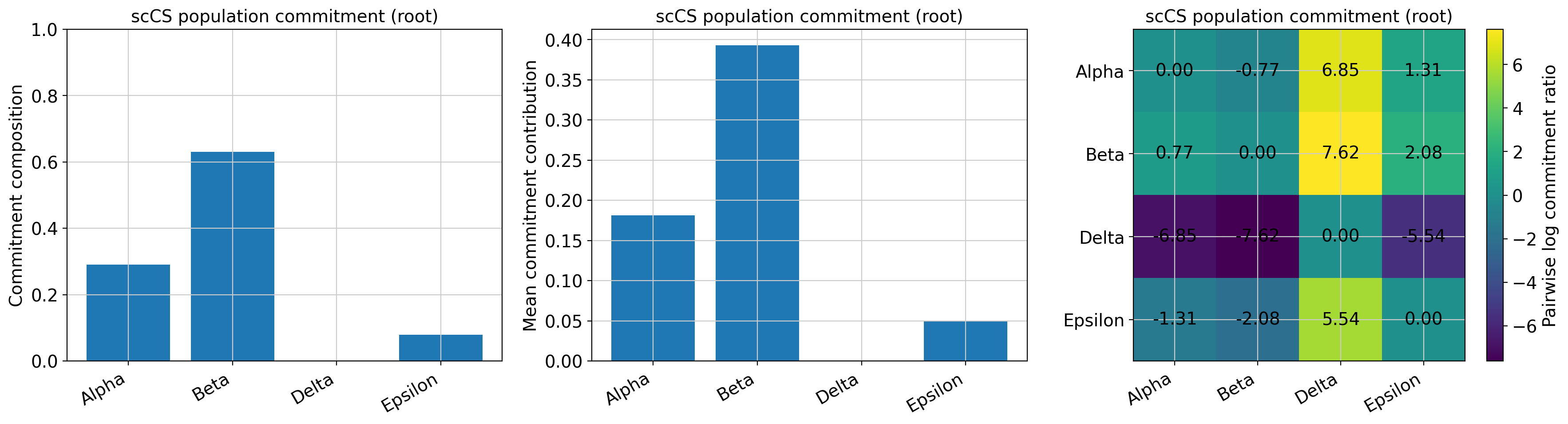
  Root future-fate composition: Alpha=0.291, Beta=0.630, Delta=0.000, Epsilon=0.079
  Solver: direct; iterations=1; residual=1.927e-15
scCS FutureFateScoreResult
  Furcation: root -> ['Alpha', 'Beta', 'Delta', 'Epsilon']
  Effective horizon: 64 (gamma=0.984615)
  Cells: 2518 selected; 1234 root
  Root affinity coverage: 1.000
  Root mean future-fate reach: 0.624
  Root mean future-fate entropy: 0.597
  Root mean future-fate specificity: 0.403
  Root mean reach-supported specificity: 0.254
  Root mean unresolved probability: 0.376
  Root mean signed progression: 0.041
  Root future-fate composition: Alpha=0.291, Beta=0.630, Delta=0.000, Epsilon=0.079
  Solver: direct; iterations=1; residual=1.927e-15

	value
0	scCS FutureFateScoreResult\n Furcation: root ...

	fate	n_anchors	mean_transition_to_same_fate_population	mean_transition_to_root	mean_transition_to_other_selected_fates	mean_signed_progression	forward_fraction
0	Alpha	49	0.998604	0.000101	0.001295	-0.039809	0.000000
1	Beta	60	1.000000	0.000000	0.000000	-0.009623	0.033333
2	Delta	10	0.857701	0.000722	0.141577	-0.042991	0.000000
3	Epsilon	15	0.686047	0.198733	0.115220	-0.098604	0.000000

6. Core star dashboard¶

All panels use identical cell positions. The star is a standardized display, not an inverse map of UMAP or gene space. The one-step selected-path coverage panel is a graph-scope diagnostic and should not be interpreted as commitment.

[7]:

fig, axes = plt.subplots(2, 4, figsize=(23, 11))
scorer.plot_star(result, color_by="population", title="Cell annotation", ax=axes[0, 0])
scorer.plot_star(result, color_by="status", title="Future-fate status", ax=axes[0, 1])
scorer.plot_star(result, color_by="future_fate_reach", title="Future-fate reach", ax=axes[0, 2])
scorer.plot_star(
    result,
    color_by="future_fate_specificity",
    title="Future-fate specificity",
    ax=axes[0, 3],
)
scorer.plot_star(
    result,
    color_by="reach_supported_specificity",
    title="Reach-supported specificity",
    ax=axes[1, 0],
)
scorer.plot_star(result, color_by="future_fate_entropy", title="Future-fate entropy", ax=axes[1, 1])
scorer.plot_star(
    result,
    color_by="signed_progression",
    title="Signed ordering progression",
    cmap="coolwarm",
    ax=axes[1, 2],
)
scorer.plot_star(
    result,
    color_by="selected_path_coverage",
    title="One-step selected-path coverage",
    ax=axes[1, 3],
)
fig.tight_layout()
fig.savefig(OUTPUT_DIR / "core_star_dashboard.png", dpi=200, bbox_inches="tight")
plt.show()

../_images/tutorials_01_pancreas_single_scorer_14_0.png

7. Fate-specific affinity and absolute contribution¶

[8]:

fig, axes = plt.subplots(2, len(FATES), figsize=(5.2 * len(FATES), 9.5))
for column, fate in enumerate(FATES):
    scorer.plot_star(
        result,
        color_by=f"future_fate_affinity:{fate}",
        title=f"Conditional affinity: {fate}",
        ax=axes[0, column],
    )
    scorer.plot_star(
        result,
        color_by=f"future_fate_contribution:{fate}",
        title=f"Absolute contribution: {fate}",
        ax=axes[1, column],
    )
fig.tight_layout()
fig.savefig(OUTPUT_DIR / "fate_affinity_and_contribution.png", dpi=200, bbox_inches="tight")
plt.show()

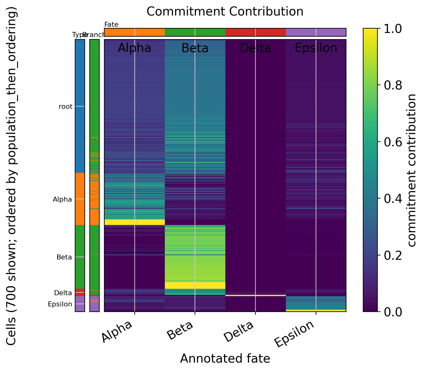
../_images/tutorials_01_pancreas_single_scorer_16_0.png

8. Cell-level heatmaps with annotation strips¶

[9]:

affinity_fig = scorer.plot_commitment_heatmap(
    result,
    metric="future_fate_affinity",
    population="all",
    sort_by="population_then_ordering",
    row_annotation=("population", "dominant_affinity"),
    show_fate_strip=True,
    max_cells=700,
)
affinity_fig.savefig(OUTPUT_DIR / "future_fate_affinity_heatmap.png", dpi=200, bbox_inches="tight")
plt.show()

contribution_fig = scorer.plot_commitment_heatmap(
    result,
    metric="future_fate_contribution",
    population="all",
    sort_by="population_then_ordering",
    row_annotation=("population", "dominant_affinity"),
    show_fate_strip=True,
    max_cells=700,
)
contribution_fig.savefig(
    OUTPUT_DIR / "future_fate_contribution_heatmap.png",
    dpi=200,
    bbox_inches="tight",
)
plt.show()

../_images/tutorials_01_pancreas_single_scorer_18_0.png

../_images/tutorials_01_pancreas_single_scorer_18_1.png

9. Population summaries, fate composition, and pairwise balance¶

[10]:

fig, axes = plt.subplots(1, 3, figsize=(18, 5))
scorer.plot_commitment_bar(
    result,
    population="root",
    metric="commitment_composition",
    ax=axes[0],
)
scorer.plot_population_commitment(
    result,
    population="root",
    metric="mean_commitment_contribution",
    ax=axes[1],
)
scorer.plot_pairwise_cs(result, population="root", ax=axes[2])
fig.tight_layout()
fig.savefig(OUTPUT_DIR / "root_population_summaries.png", dpi=200, bbox_inches="tight")
plt.show()

../_images/tutorials_01_pancreas_single_scorer_20_0.png

10. Branch behavior and ordering thirds¶

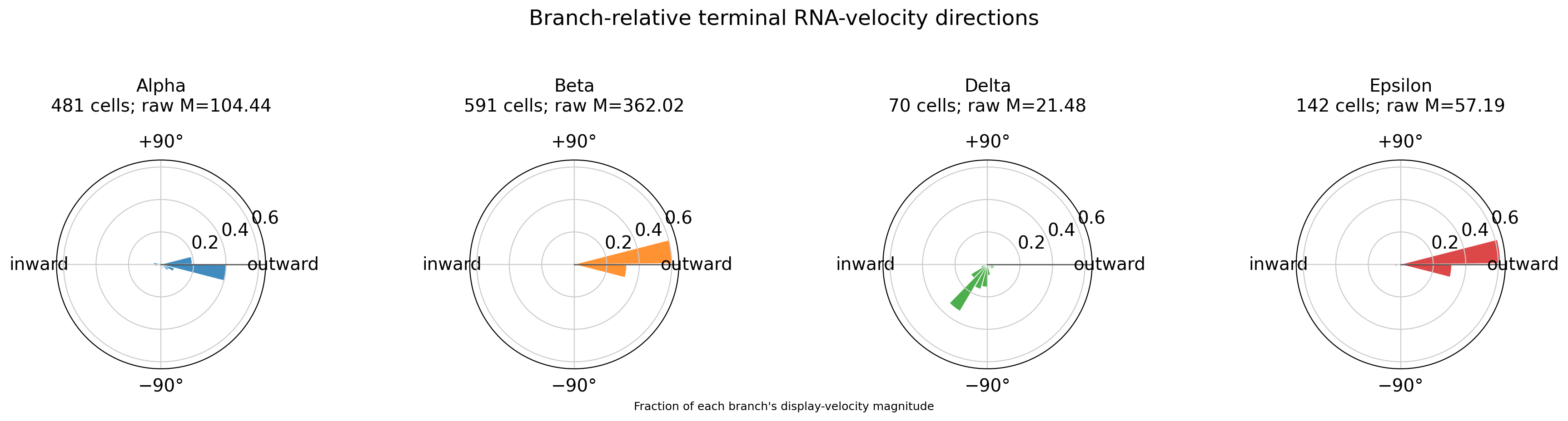
A branch can retain strong fate identity while signed progression turns negative. This is particularly important for the curved Alpha path and the unusual Delta and Epsilon velocity fields.

[11]:

selected = adata.obs.loc[result.cell_ids].copy()
selected["future_fate_reach"] = result.future_fate_reach
selected["future_fate_specificity"] = result.future_fate_specificity
selected["reach_supported_specificity"] = result.reach_supported_specificity
selected["signed_progression"] = result.signed_progression
selected["ordering_third"] = ordering_thirds(selected[ORDERING_KEY].to_numpy(float))
for fate_index, fate in enumerate(FATES):
    selected[f"affinity_{fate}"] = result.future_fate_affinity[:, fate_index]
    selected[f"contribution_{fate}"] = result.future_fate_contribution[:, fate_index]

population_summary = selected.groupby("clusters", observed=True).agg(
    n_cells=("future_fate_reach", "size"),
    mean_reach=("future_fate_reach", "mean"),
    mean_specificity=("future_fate_specificity", "mean"),
    mean_supported_specificity=("reach_supported_specificity", "mean"),
    mean_progression=("signed_progression", "mean"),
    forward_fraction=("signed_progression", lambda values: float(np.mean(values > 0))),
)
display(population_summary)
population_summary.to_csv(OUTPUT_DIR / "population_summary.csv")

branch_thirds = (
    selected[selected["clusters"].astype(str).isin(FATES)]
    .groupby(["clusters", "ordering_third"], observed=True)
    .agg(
        n_cells=("future_fate_reach", "size"),
        mean_reach=("future_fate_reach", "mean"),
        mean_specificity=("future_fate_specificity", "mean"),
        mean_progression=("signed_progression", "mean"),
        forward_fraction=("signed_progression", lambda values: float(np.mean(values > 0))),
    )
)
display(branch_thirds)
branch_thirds.to_csv(OUTPUT_DIR / "branch_ordering_thirds.csv")

	n_cells	mean_reach	mean_specificity	mean_supported_specificity	mean_progression	forward_fraction
clusters
Ngn3 high EP	642	0.586236	0.389054	0.228086	0.033081	0.968847
Pre-endocrine	592	0.665058	0.417348	0.281243	0.048918	0.645270
Beta	591	0.821739	0.931207	0.771859	0.096513	0.844332
Alpha	481	0.661622	0.594197	0.411253	0.003379	0.446985
Delta	70	0.769183	0.557608	0.450258	-0.134738	0.071429
Epsilon	142	0.617827	0.500247	0.332878	0.023334	0.584507

		n_cells	mean_reach	mean_specificity	mean_progression	forward_fraction
clusters	ordering_third
Beta	early	11	0.745487	0.658780	0.143923	1.000000
	late	282	0.869033	0.999996	0.032950	0.765957
	middle	298	0.779799	0.876167	0.154913	0.912752
Alpha	late	306	0.682022	0.636212	-0.046457	0.192810
Alpha	middle	175	0.625950	0.520729	0.090521	0.891429
Delta	early	1	0.686064	0.391010	0.176562	1.000000
	late	60	0.780078	0.569959	-0.157537	0.000000
	middle	9	0.705788	0.493782	-0.017337	0.444444
Epsilon	early	1	0.658172	0.271163	0.126989	1.000000
	late	78	0.651685	0.566368	-0.034055	0.269231
	middle	63	0.575268	0.422019	0.092743	0.968254

11. Display-only RNA-velocity diagnostics¶

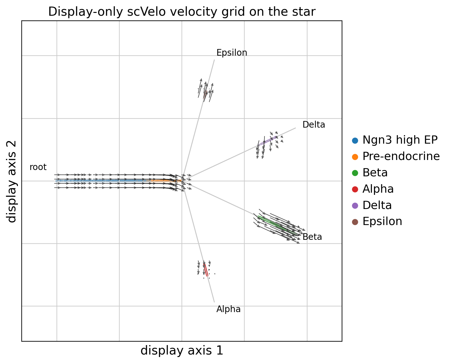
The primary scCS result above is the discounted future-fate model. The figures below are optional RNA-velocity quality-control views. They use a separate instantaneous scorer and therefore do not define future-fate affinity, reach, specificity, or entropy.

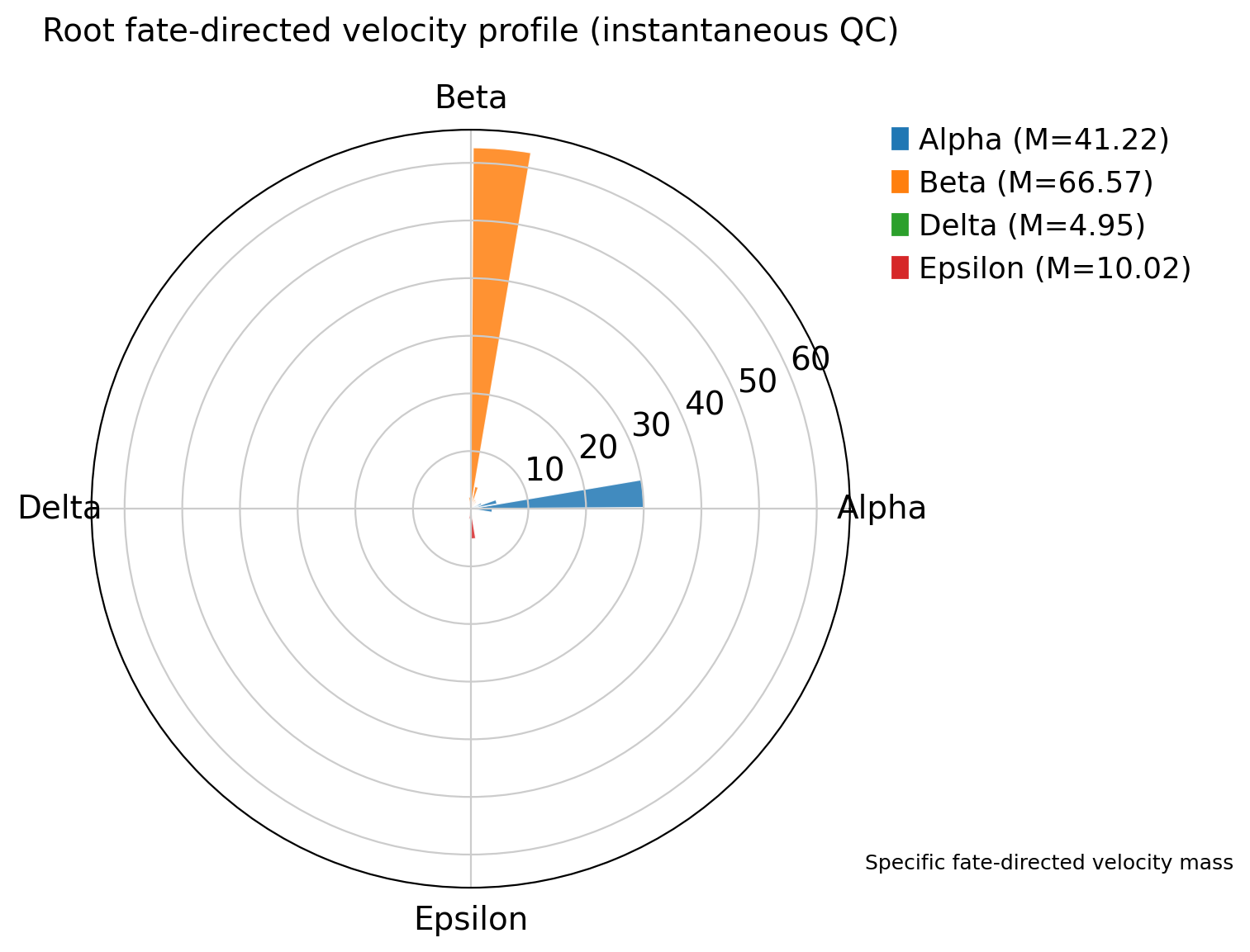
A straight star cannot preserve every turn or loop of the original manifold. We therefore show (1) the native scVelo projection on the star, (2) a root fate-directed rose after removing incoming-root progression, and (3) separate branch-relative roses in which each annotated terminal population retains its identity. In the branch-relative panels, outward is 0°, transverse motion is ±90°, and inward motion is 180°.

[12]:

# First summarize the scientific future-fate result. This table and the root
# future-fate composition plot answer which fate is dominant. Display-space
# arrows answer a different question and can be curved or retrograde.
terminal_labels = np.asarray(result.embedding.selected_labels).astype(str)
terminal_qc_rows = []
for fate_index, fate in enumerate(FATES):
    fate_mask = result.terminal_mask & (terminal_labels == fate)
    terminal_qc_rows.append(
        {
            "fate": fate,
            "n_cells": int(fate_mask.sum()),
            "mean_own_future_fate_affinity": float(
                np.nanmean(result.future_fate_affinity[fate_mask, fate_index])
            ),
            "mean_future_fate_reach": float(np.nanmean(result.future_fate_reach[fate_mask])),
            "mean_signed_progression": float(np.nanmean(result.signed_progression[fate_mask])),
        }
    )
display(pd.DataFrame(terminal_qc_rows).set_index("fate"))

# Build a separate instantaneous scorer only for RNA-velocity display QC.
# This does not alter the primary discounted future-fate result.
instantaneous_display_scorer = scCS.SingleScorer(
    adata,
    root=ROOT,
    branches=FATES,
    obs_key="clusters",
)
instantaneous_display_scorer.build_embedding(
    ordering_metric=ORDERING_KEY,
    write_to_adata=True,
    verbose=False,
)
instantaneous_display_scorer.fit(scoring_mode="instantaneous", verbose=False)
instantaneous_display_result = instantaneous_display_scorer.score(
    write_to_adata=False,
    verbose=False,
)

# Native scVelo projection onto the straightened star. Curved, loop-like, or
# retrograde source trajectories can therefore look inward on some branches.
fig, ax = plt.subplots(figsize=(8, 6))
instantaneous_display_scorer.plot_velocity_embedding_grid(
    instantaneous_display_result,
    population="all",
    density=0.9,
    smooth=0.55,
    min_mass=1.0,
    n_neighbors=50,
    projection_mode="scvelo",
    title="Display-only scVelo velocity grid on the star",
    ax=ax,
)
fig.tight_layout()
fig.savefig(OUTPUT_DIR / "display_velocity_grid.png", dpi=200, bbox_inches="tight")
plt.show()

# Root fate-directed velocity after removing incoming-root progression. This
# is the closest analogue of the familiar binned commitment rose and does not
# assign the incoming root direction to a terminal sector.
root_rose = plt.figure(figsize=(8.5, 6.5))
root_rose_ax = root_rose.add_subplot(111, projection="polar")
instantaneous_display_scorer.plot_rose(
    instantaneous_display_result,
    population="root",
    mode="branch",
    n_bins=36,
    normalization="mass",
    title="Root fate-directed velocity profile (instantaneous QC)",
    ax=root_rose_ax,
)
root_rose.subplots_adjust(right=0.72)
root_rose.savefig(OUTPUT_DIR / "root_branch_velocity_rose.png", dpi=200, bbox_inches="tight")
plt.show()

# Terminal branches are shown separately. Each panel keeps cells attached to
# their annotated branch: 0° is outward, ±90° is transverse, and 180° is
# inward. Thus a retrograde Delta, Epsilon, or Gut vector is never relabeled as
# movement toward a different fate merely because of the 2D star layout.
branch_profiles = instantaneous_display_scorer.plot_branch_velocity_profiles(
    instantaneous_display_result,
    n_bins=24,
    normalization="within_branch",
    projection_mode="scvelo",
    title="Branch-relative terminal RNA-velocity directions",
)
branch_profiles.savefig(
    OUTPUT_DIR / "branch_relative_velocity_profiles.png",
    dpi=200,
    bbox_inches="tight",
)
plt.show()

	n_cells	mean_own_future_fate_affinity	mean_future_fate_reach	mean_signed_progression
fate
Alpha	481	0.733023	0.661622	0.003379
Beta	591	0.963389	0.821739	0.096513
Delta	70	0.180194	0.769183	-0.134738
Epsilon	142	0.733876	0.617827	0.023334

computing velocity embedding
    finished (0:00:00)

../_images/tutorials_01_pancreas_single_scorer_24_2.png

../_images/tutorials_01_pancreas_single_scorer_24_3.png

computing velocity embedding
    finished (0:00:00)

../_images/tutorials_01_pancreas_single_scorer_24_5.png

12. Gene expression on the star¶

[13]:

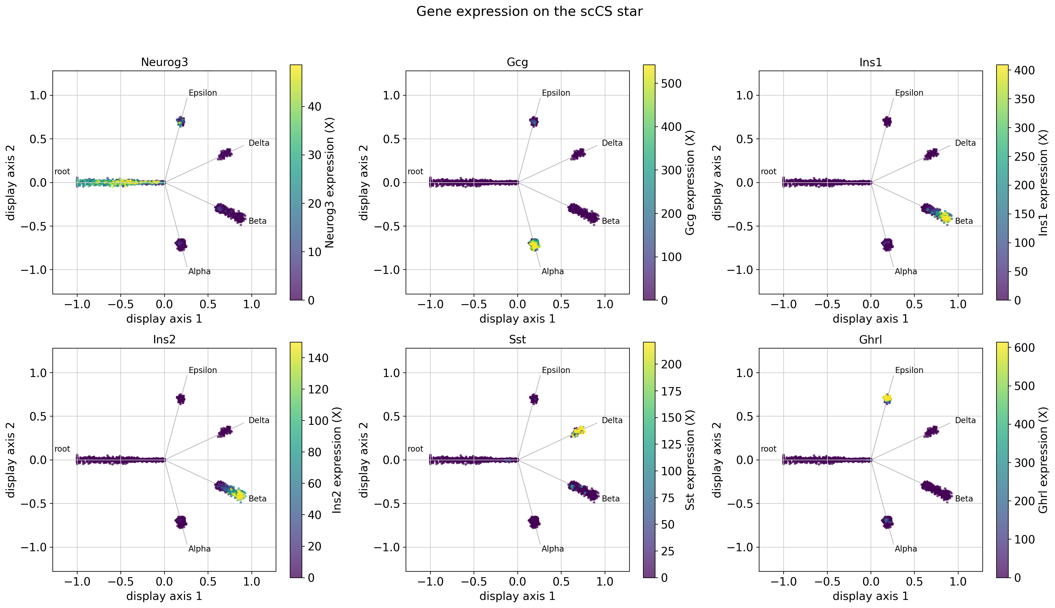
marker_candidates = ["Neurog3", "Gcg", "Ins1", "Ins2", "Sst", "Ghrl"]
markers, missing_markers = resolve_present_genes(adata, marker_candidates)
print("Resolved markers:", markers)
print("Missing markers:", missing_markers)
if markers:
    marker_fig = scorer.plot_gene_expression_star(
        markers,
        result,
        terminal_layout="ordering",
        ncols=3,
        shared_scale=False,
    )
    marker_fig.savefig(OUTPUT_DIR / "marker_expression_stars.png", dpi=200, bbox_inches="tight")
    plt.show()

Resolved markers: ['Neurog3', 'Gcg', 'Ins1', 'Ins2', 'Sst', 'Ghrl']
Missing markers: []

../_images/tutorials_01_pancreas_single_scorer_26_1.png

13. Expression trends along the supplied ordering¶

[14]:

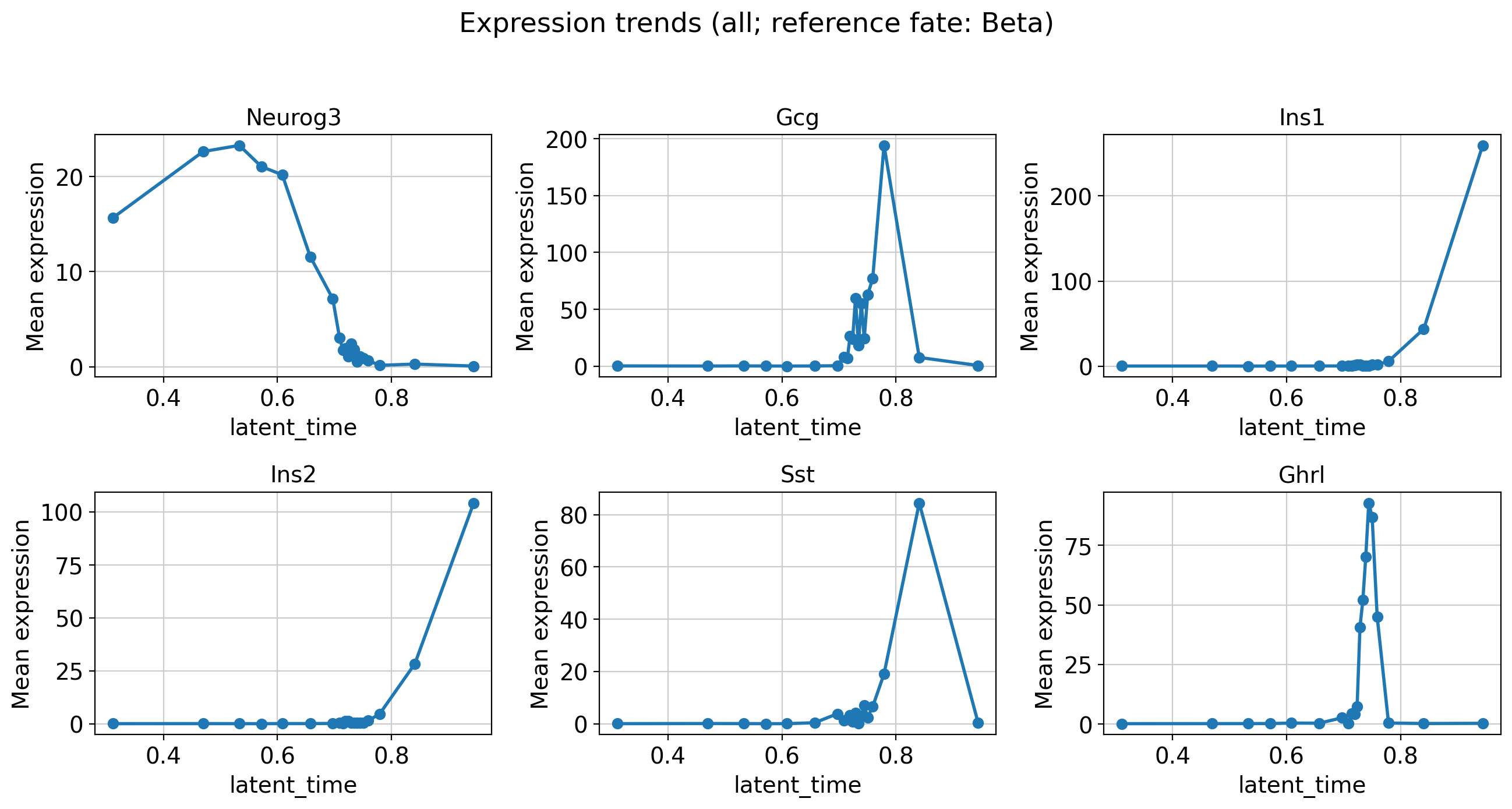
if markers:
    trend_fig = scorer.plot_expression_trends(
        markers,
        result,
        x_axis="ordering",
        population="all",
        n_bins=20,
        ncols=3,
    )
    trend_fig.savefig(OUTPUT_DIR / "marker_expression_trends.png", dpi=200, bbox_inches="tight")
    plt.show()

../_images/tutorials_01_pancreas_single_scorer_28_0.png

14. Candidate genes associated with future-fate outputs¶

Cell-level associations are exploratory because cells are not independent biological replicates. Use inference_unit="replicate" only when a valid independent replicate column exists and enough units pass the minimum-cell filter. Associations are candidates, not causal lineage drivers.

[15]:

association = scorer.get_commitment_associated_genes(
    outcome="future_fate_affinity",
    fate_names=FATES,
    population="root",
    inference_unit="cell_exploratory",
    pseudotime_key=ORDERING_KEY,
    min_cells=100,
    min_feature_cells=10,
    min_feature_fraction=0.01,
    n_top_genes=30,
    verbose=True,
)
for fate in FATES:
    print("\n", fate)
    display(association.top(fate, n=15))
association.export(OUTPUT_DIR, prefix="future_fate_gene_association")


[scCS] Candidate commitment-associated genes: Alpha
        inference_unit=cell_exploratory; matrix=X; n_units=1234; tested_genes=6946
 rank    gene   effect   pvalue_adj  significant
    1  Tmsb4x 0.275744 6.866232e-20         True
    2 Neurog3 0.249886 5.188467e-16         True
    3    Ppib 0.242993 3.842847e-15         True
    4     Mdk 0.242233 4.414893e-15         True
    5    Rps9 0.239684 9.050625e-15         True
    6     Cck 0.234886 2.988312e-14         True
    7    Btg2 0.233772 3.955025e-14         True
    8  Btbd17 0.233522 4.020746e-14         True
    9    Cd63 0.229856 1.163901e-13         True
   10 Igfbpl1 0.225002 4.719493e-13         True
   11   Rps11 0.220966 1.330870e-12         True
   12 Gadd45a 0.218992 2.158346e-12         True
   13    Pax4 0.214899 6.643259e-12         True
   14    Cdk4 0.208052 3.532527e-11         True
   15    Dbn1 0.203733 1.012706e-10         True
   16 Smarcd2 0.202143 1.460725e-10         True
   17    Selm 0.200973 1.935800e-10         True
   18    Tecr 0.199264 2.884216e-10         True
   19   Cldn6 0.197887 3.750920e-10         True
   20    Rps5 0.195899 6.087173e-10         True
   21    Rps8 0.193160 1.193368e-09         True
   22   Rps19 0.192583 1.350683e-09         True
   23   Rpl32 0.192380 1.387809e-09         True
   24  Rpl18a 0.192309 1.387809e-09         True
   25  Ifitm2 0.185488 6.752053e-09         True
   26  Rpl37a 0.183151 1.121243e-08         True
   27    Npc2 0.182841 1.186314e-08         True
   28   Rps23 0.181245 1.674072e-08         True
   29  Hpcal1 0.178260 3.310284e-08         True
   30   Cotl1 0.176209 5.144636e-08         True

[scCS] Candidate commitment-associated genes: Beta
        inference_unit=cell_exploratory; matrix=X; n_units=1234; tested_genes=6946
 rank          gene   effect   pvalue_adj  significant
    1         Pcsk2 0.240656 3.654280e-14         True
    2          Rbp4 0.224756 3.213982e-12         True
    3        Npepl1 0.218365 1.550325e-11         True
    4          Pdx1 0.216645 2.026609e-11         True
    5          Mnx1 0.215440 2.376480e-11         True
    6          Pim2 0.195233 4.638021e-09         True
    7 1700086L19Rik 0.187750 2.629641e-08         True
    8           Pyy 0.183906 5.927710e-08         True
    9         Fxyd6 0.180545 1.184303e-07         True
   10          Chgb 0.178527 1.725473e-07         True
   11          Gnas 0.176425 2.570263e-07         True
   12       S100a11 0.175677 2.816025e-07         True
   13        Pcsk1n 0.170399 8.578265e-07         True
   14         Gng12 0.168234 1.289587e-06         True
   15        Elmod1 0.163479 3.172835e-06         True
   16         Prps1 0.157899 9.108764e-06         True
   17         Anxa4 0.156565 1.089599e-05         True
   18        Sec61b 0.155863 1.191686e-05         True
   19         Syt13 0.152620 2.184586e-05         True
   20       Fam159b 0.152054 2.342385e-05         True
   21        Cryba2 0.149606 3.635226e-05         True
   22          Xist 0.144618 8.142971e-05         True
   23        Klhl32 0.139189 2.147447e-04         True
   24        Papss2 0.138580 2.320391e-04         True
   25      Slc16a12 0.138162 2.350279e-04         True
   26         Flrt1 0.137802 2.434007e-04         True
   27           Fev 0.131738 6.324788e-04         True
   28         Ndc80 0.129850 8.094011e-04         True
   29        Nkx6-1 0.128587 9.539775e-04         True
   30       Hdgfrp3 0.127068 1.172122e-03         True

[scCS] Candidate commitment-associated genes: Delta
        inference_unit=cell_exploratory; matrix=X; n_units=1234; tested_genes=6946
 rank      gene   effect   pvalue_adj  significant
    1    Cdkn1a 0.341412 3.418676e-31         True
    2    Mboat4 0.338549 6.680157e-31         True
    3      Isl1 0.297690 2.019228e-23         True
    4       Arx 0.297191 2.019228e-23         True
    5     Cd200 0.287990 6.507125e-22         True
    6      Peg3 0.269294 6.235222e-19         True
    7    Tm4sf4 0.249135 5.823501e-16         True
    8     Peg10 0.233154 6.379363e-14         True
    9 Trp53cor1 0.228891 2.157446e-13         True
   10     Glud1 0.214502 1.092584e-11         True
   11      Muc1 0.208587 4.785118e-11         True
   12  Trp53i13 0.206268 8.553140e-11         True
   13      Arg1 0.202316 2.151444e-10         True
   14  Slc16a10 0.202032 2.225874e-10         True
   15     Syne1 0.199276 4.409085e-10         True
   16     Anpep 0.182326 2.592032e-08         True
   17      Hhex 0.178956 5.368210e-08         True
   18     Alcam 0.171484 2.706560e-07         True
   19      Gch1 0.169114 4.310142e-07         True
   20     Mctp2 0.164925 1.042353e-06         True
   21    Nap1l5 0.162142 1.789696e-06         True
   22      Zim1 0.158269 3.818520e-06         True
   23     Sfxn2 0.156223 5.667354e-06         True
   24     Rgs17 0.154249 8.250985e-06         True
   25   Eif2s3y 0.153502 9.367439e-06         True
   26      Hadh 0.144885 4.491779e-05         True
   27  Hepacam2 0.144025 5.176745e-05         True
   28   Fam183b 0.137796 1.506197e-04         True
   29      Cd47 0.137416 1.583615e-04         True
   30       Ghr 0.136067 1.974891e-04         True

[scCS] Candidate commitment-associated genes: Epsilon
        inference_unit=cell_exploratory; matrix=X; n_units=1234; tested_genes=6946
 rank      gene   effect   pvalue_adj  significant
    1    Cdkn1a 0.309303 6.677054e-25         True
    2       Arx 0.303512 3.788425e-24         True
    3    Mboat4 0.290981 4.025278e-22         True
    4    Tm4sf4 0.237835 2.868121e-14         True
    5      Peg3 0.237758 2.868121e-14         True
    6     Glud1 0.237460 2.868121e-14         True
    7     Cd200 0.229925 1.865291e-13         True
    8 Trp53cor1 0.211789 2.642934e-11         True
    9      Muc1 0.208200 6.648502e-11         True
   10     Anpep 0.187485 1.181492e-08         True
   11      Isl1 0.183961 2.461173e-08         True
   12      Arg1 0.183844 2.461173e-08         True
   13    Nap1l5 0.172484 2.901449e-07         True
   14  Trp53i13 0.159244 4.842869e-06         True
   15     Mctp2 0.158913 4.842869e-06         True
   16     Alcam 0.156351 7.914514e-06         True
   17  Slc16a10 0.145347 6.052592e-05         True
   18     Gsta3 0.144897 6.224458e-05         True
   19     Peg10 0.143662 7.637226e-05         True
   20      Zim1 0.142210 9.493699e-05         True
   21       Bsg 0.141145 1.099295e-04         True
   22    Grin3a 0.138595 1.586106e-04         True
   23 Serpina1c 0.138225 1.631704e-04         True
   24     Sfxn2 0.135531 2.432142e-04         True
   25     Syne1 0.135229 2.515859e-04         True
   26      Irx2 0.134787 2.668251e-04         True
   27     Gria2 0.131847 4.160088e-04         True
   28     Anxa2 0.131817 4.160088e-04         True
   29     Acot1 0.128322 6.409868e-04         True
   30      Dll1 0.127325 7.461387e-04         True

 Alpha

	gene	effect	pvalue	pvalue_adj	feature_mean	feature_sd	n_detected_cells	n_units	significant	absolute_effect	rank
0	Tmsb4x	0.275744	5.931096e-23	6.866232e-20	26.480909	25.720442	1169	1234	True	0.275744	1
1	Neurog3	0.249886	5.228804e-19	5.188467e-16	13.379286	13.727636	988	1234	True	0.249886	2
2	Ppib	0.242993	4.979215e-18	3.842847e-15	8.263345	5.597094	1201	1234	True	0.242993	3
3	Mdk	0.242233	6.356023e-18	4.414893e-15	15.501658	12.948563	1124	1234	True	0.242233	4
4	Rps9	0.239684	1.433298e-17	9.050625e-15	32.504977	9.654044	1234	1234	True	0.239684	5
5	Cck	0.234886	6.453309e-17	2.988312e-14	20.157887	22.982749	994	1234	True	0.234886	6
6	Btg2	0.233772	9.110337e-17	3.955025e-14	8.378012	5.691946	1196	1234	True	0.233772	7
7	Btbd17	0.233522	9.840581e-17	4.020746e-14	5.285445	5.445983	882	1234	True	0.233522	8
8	Cd63	0.229856	3.016156e-16	1.163901e-13	10.626693	5.767550	1221	1234	True	0.229856	9
9	Igfbpl1	0.225002	1.290964e-15	4.719493e-13	2.379176	3.276287	703	1234	True	0.225002	10
10	Rps11	0.220966	4.215253e-15	1.330870e-12	22.155707	7.528621	1234	1234	True	0.220966	11
11	Gadd45a	0.218992	7.457573e-15	2.158346e-12	6.003202	7.458282	832	1234	True	0.218992	12
12	Pax4	0.214899	2.391038e-14	6.643259e-12	2.811147	2.896685	863	1234	True	0.214899	13
13	Cdk4	0.208052	1.594313e-13	3.532527e-11	7.591262	4.271979	1200	1234	True	0.208052	14
14	Dbn1	0.203733	5.102894e-13	1.012706e-10	2.202929	2.235892	888	1234	True	0.203733	15


 Beta

	gene	effect	pvalue	pvalue_adj	feature_mean	feature_sd	n_detected_cells	n_units	significant	absolute_effect	rank
0	Pcsk2	0.240656	1.052197e-17	3.654280e-14	0.824410	2.119913	285	1234	True	0.240656	1
1	Rbp4	0.224756	1.388129e-15	3.213982e-12	6.374880	17.573840	573	1234	True	0.224756	2
2	Npepl1	0.218365	8.927872e-15	1.550325e-11	1.879040	2.161760	844	1234	True	0.218365	3
3	Pdx1	0.216645	1.458831e-14	2.026609e-11	1.220922	1.919877	586	1234	True	0.216645	4
4	Mnx1	0.215440	2.052819e-14	2.376480e-11	0.251422	0.889925	125	1234	True	0.215440	5
5	Pim2	0.195233	4.674078e-12	4.638021e-09	0.999573	1.959778	460	1234	True	0.195233	6
6	1700086L19Rik	0.187750	3.028669e-11	2.629641e-08	1.625739	3.346094	461	1234	True	0.187750	7
7	Pyy	0.183906	7.680592e-11	5.927710e-08	15.748496	61.305059	631	1234	True	0.183906	8
8	Fxyd6	0.180545	1.705015e-10	1.184303e-07	0.975067	1.746535	455	1234	True	0.180545	9
9	Chgb	0.178527	2.732536e-10	1.725473e-07	26.170255	48.147127	615	1234	True	0.178527	10
10	Gnas	0.176425	4.440420e-10	2.570263e-07	24.092879	17.366661	1234	1234	True	0.176425	11
11	S100a11	0.175677	5.270417e-10	2.816025e-07	2.517067	2.615982	914	1234	True	0.175677	12
12	Pcsk1n	0.170399	1.728991e-09	8.578265e-07	3.587842	6.484170	558	1234	True	0.170399	13
13	Gng12	0.168234	2.784883e-09	1.289587e-06	0.531641	1.061274	355	1234	True	0.168234	14
14	Elmod1	0.163479	7.765361e-09	3.172835e-06	0.060351	0.287795	57	1234	True	0.163479	15


 Delta

	gene	effect	pvalue	pvalue_adj	feature_mean	feature_sd	n_detected_cells	n_units	significant	absolute_effect	rank
0	Cdkn1a	0.341412	4.921791e-35	3.418676e-31	7.192985	11.485302	930	1234	True	0.341412	1
1	Mboat4	0.338549	1.923454e-34	6.680157e-31	0.244339	1.053657	119	1234	True	0.338549	2
2	Isl1	0.297690	1.187606e-26	2.019228e-23	3.723734	8.049448	438	1234	True	0.297690	3
3	Arx	0.297191	1.453519e-26	2.019228e-23	0.548678	1.612283	209	1234	True	0.297191	4
4	Cd200	0.287990	5.620897e-25	6.507125e-22	0.846095	1.491867	425	1234	True	0.287990	5
5	Peg3	0.269294	6.283696e-22	6.235222e-19	5.624904	5.022496	1143	1234	True	0.269294	6
6	Tm4sf4	0.249135	6.707171e-19	5.823501e-16	3.366878	4.171071	862	1234	True	0.249135	7
7	Peg10	0.233154	1.102107e-16	6.379363e-14	0.182685	0.908079	72	1234	True	0.233154	8
8	Trp53cor1	0.228891	4.037835e-16	2.157446e-13	0.106156	0.414571	95	1234	True	0.228891	9
9	Glud1	0.214502	2.674047e-14	1.092584e-11	3.630171	4.123165	972	1234	True	0.214502	10
10	Muc1	0.208587	1.377805e-13	4.785118e-11	0.439841	0.891349	326	1234	True	0.208587	11
11	Trp53i13	0.206268	2.585890e-13	8.553140e-11	0.562178	1.028628	403	1234	True	0.206268	12
12	Arg1	0.202316	7.433724e-13	2.151444e-10	0.135893	0.751025	83	1234	True	0.202316	13
13	Slc16a10	0.202032	8.011352e-13	2.225874e-10	0.061193	0.363854	45	1234	True	0.202032	14
14	Syne1	0.199276	1.650392e-12	4.409085e-10	0.107190	0.437560	87	1234	True	0.199276	15


 Epsilon

	gene	effect	pvalue	pvalue_adj	feature_mean	feature_sd	n_detected_cells	n_units	significant	absolute_effect	rank
0	Cdkn1a	0.309303	9.612805e-29	6.677054e-25	7.192985	11.485302	930	1234	True	0.309303	1
1	Arx	0.303512	1.090822e-27	3.788425e-24	0.548678	1.612283	209	1234	True	0.303512	2
2	Mboat4	0.290981	1.738531e-25	4.025278e-22	0.244339	1.053657	119	1234	True	0.290981	3
3	Tm4sf4	0.237835	2.569547e-17	2.868121e-14	3.366878	4.171071	862	1234	True	0.237835	4
4	Peg3	0.237758	2.632457e-17	2.868121e-14	5.624904	5.022496	1143	1234	True	0.237758	5
5	Glud1	0.237460	2.890418e-17	2.868121e-14	3.630171	4.123165	972	1234	True	0.237460	6
6	Cd200	0.229925	2.953960e-16	1.865291e-13	0.846095	1.491867	425	1234	True	0.229925	7
7	Trp53cor1	0.211789	5.707460e-14	2.642934e-11	0.106156	0.414571	95	1234	True	0.211789	8
8	Muc1	0.208200	1.531472e-13	6.648502e-11	0.439841	0.891349	326	1234	True	0.208200	9
9	Anpep	0.187485	3.231839e-11	1.181492e-08	0.294801	0.849643	224	1234	True	0.187485	10
10	Isl1	0.183961	7.580492e-11	2.461173e-08	3.723734	8.049448	438	1234	True	0.183961	11
11	Arg1	0.183844	7.795250e-11	2.461173e-08	0.135893	0.751025	83	1234	True	0.183844	12
12	Nap1l5	0.172484	1.086059e-09	2.901449e-07	0.037859	0.316134	27	1234	True	0.172484	13
13	Trp53i13	0.159244	1.888294e-08	4.842869e-06	0.562178	1.028628	403	1234	True	0.159244	14
14	Mctp2	0.158913	2.021929e-08	4.842869e-06	0.017739	0.159846	17	1234	True	0.158913	15

[15]:

['tutorial_outputs/pancreas_single/future_fate_gene_association_Alpha.csv',
 'tutorial_outputs/pancreas_single/future_fate_gene_association_Beta.csv',
 'tutorial_outputs/pancreas_single/future_fate_gene_association_Delta.csv',
 'tutorial_outputs/pancreas_single/future_fate_gene_association_Epsilon.csv',
 'tutorial_outputs/pancreas_single/future_fate_gene_association_metadata.json']

15. Terminal annotation markers¶

[16]:

fate_markers = scorer.get_fate_markers(
    n_genes=50,
    fdr_threshold=0.05,
    logfc_threshold=0.25,
    min_cells=10,
    verbose=True,
)
for fate, table in fate_markers.items():
    print("\n", fate)
    display(table.head(15))
    table.to_csv(OUTPUT_DIR / f"terminal_markers_{fate}.csv", index=False)

ranking genes
    finished (0:00:00)

[scCS] Fate markers: Alpha vs root; significant=50
 rank    gene  logfoldchange    pvalue_adj
    1     Pyy     233.343811 1.051944e-160
    2     Gcg     209.721115  1.613987e-83
    3    Iapp     100.156334 3.267432e-138
    4     Ttr      69.962547 3.499607e-146
    5    Gnas      51.120472 2.153794e-130
    6    Rbp4      43.370220 7.934233e-127
    7  Tmem27      18.768389 3.627194e-200
    8 Slc38a5      18.712347 1.562776e-124
    9  Pcsk1n      17.453619 6.113637e-142
   10     Cpe      13.869763 1.434444e-125
   11 Slc25a5      12.463739  3.970180e-52
   12    Gast      11.470784  3.008741e-52
   13   Pcsk2       9.351954 1.479988e-117
   14    Gpx3       8.338355 3.580264e-131
   15   Meis2       8.270338 1.147131e-145
   16   Peg10       7.708434  2.012753e-97
   17    Isl1       7.264405  2.414985e-71
   18    Ssr2       6.711359 2.825360e-103
   19 Tmsb15l       6.403490 1.952847e-101
   20  Tspan7       6.041723 1.076545e-122
ranking genes
    finished (0:00:00)

[scCS] Fate markers: Beta vs root; significant=50
 rank          gene  logfoldchange    pvalue_adj
    1          Iapp     186.131287 1.182187e-212
    2           Pyy     162.698456 1.170819e-166
    3          Rbp4      50.622169 2.567789e-195
    4          Ins2      48.017612  9.881409e-92
    5          Gnas      42.680595 7.839004e-158
    6          Nnat      42.575066 3.539079e-142
    7           Ttr      25.199047  7.322854e-82
    8        Sec61b      13.772089 1.602273e-188
    9          Dlk1      13.032376 4.344538e-143
   10        Pcsk1n      11.741943 4.973997e-133
   11       Ppp1r1a      11.731724 5.904462e-129
   12         Pcsk2      10.887548 2.477486e-210
   13       Slc38a5       8.947008 5.318520e-109
   14           Cpe       8.691454  3.550664e-97
   15         Hspa5       8.391294 3.347481e-145
   16 1700086L19Rik       8.083915 1.325254e-145
   17          Ssr2       7.868492 3.666202e-142
   18        Sdf2l1       7.639710 6.866010e-115
   19         Gng12       7.454716 1.473717e-180
   20        Tuba1a       6.965763  2.175403e-94
ranking genes
    finished (0:00:00)

[scCS] Fate markers: Delta vs root; significant=50
 rank    gene  logfoldchange   pvalue_adj
    1     Pyy     507.735718 1.707881e-38
    2     Sst     333.075989 3.239883e-31
    3    Rbp4     204.135147 3.087391e-40
    4    Iapp     103.372108 3.450474e-38
    5    Hhex      18.528818 2.771210e-36
    6    Dlk1      17.492176 3.239883e-31
    7   Cd24a      17.178232 9.241425e-29
    8    Gnas      16.492489 1.108358e-09
    9    Isl1      14.357853 2.157751e-24
   10    Gpx3      10.721635 2.015825e-30
   11    Ssr2      10.476543 9.734139e-28
   12   Pcsk2      10.011806 2.975781e-28
   13    Hadh       9.676562 2.701236e-34
   14    Arg1       9.438912 6.021122e-32
   15 Fam183b       8.570268 5.275840e-25
   16   Meis2       7.521049 5.229345e-28
   17 Fam159b       7.400708 2.537471e-10
   18  Tmem27       7.314791 2.373473e-22
   19   Kctd8       6.747847 1.584258e-11
   20    Mest       6.589624 1.620312e-18
ranking genes
    finished (0:00:00)

[scCS] Fate markers: Epsilon vs root; significant=50
 rank    gene  logfoldchange   pvalue_adj
    1    Ghrl     496.845154 1.711900e-80
    2     Pyy     105.076279 1.520765e-33
    3    Rbp4      84.230026 1.166756e-63
    4  Lrpprc      26.874617 2.212602e-35
    5    Isl1      23.863163 5.599882e-57
    6    Iapp      19.742641 2.165407e-31
    7  Maged2      16.161346 1.336546e-53
    8     Bsg      13.106299 2.802268e-52
    9 Slc38a5      10.352853 2.793423e-28
   10  Tmem27      10.297958 4.252569e-35
   11   Hspa5       9.316794 1.551241e-41
   12   Itm2b       8.679244 9.753602e-37
   13 Fam183b       8.656516 3.120110e-44
   14    Ssr2       8.275435 4.458118e-48
   15    Arg1       7.801110 3.470800e-39
   16    Irx2       6.467189 1.281201e-32
   17 Gm11837       6.296493 6.988201e-26
   18   Anpep       5.762079 5.298260e-40
   19  Sdf2l1       5.160809 3.525051e-33
   20    Ssr4       4.953045 8.442124e-37

 Alpha

	gene	score	logfoldchange	pvalue	pvalue_adj	pct_terminal	significant	analysis_type	rank
0	Pyy	27.298784	233.343811	4.384929e-164	1.051944e-160	0.968815	True	terminal_annotation_marker_vs_root	1
1	Gcg	19.606232	209.721115	1.367976e-85	1.613987e-83	0.656965	True	terminal_annotation_marker_vs_root	2
2	Iapp	25.275759	100.156334	5.901990e-141	3.267432e-138	0.854470	True	terminal_annotation_marker_vs_root	3
3	Ttr	26.014395	69.962547	3.403814e-149	3.499607e-146	1.000000	True	terminal_annotation_marker_vs_root	4
4	Gnas	24.545862	51.120472	4.788205e-133	2.153794e-130	1.000000	True	terminal_annotation_marker_vs_root	5
5	Rbp4	24.200369	43.370220	2.204872e-129	7.934233e-127	0.962578	True	terminal_annotation_marker_vs_root	6
6	Tmem27	30.478390	18.768389	5.039869e-204	3.627194e-200	0.981289	True	terminal_annotation_marker_vs_root	7
7	Slc38a5	23.975632	18.712347	4.994283e-127	1.562776e-124	0.920998	True	terminal_annotation_marker_vs_root	8
8	Pcsk1n	25.622826	17.453619	8.494702e-145	6.113637e-142	0.997921	True	terminal_annotation_marker_vs_root	9
9	Cpe	24.078638	13.869763	4.185540e-128	1.434444e-125	1.000000	True	terminal_annotation_marker_vs_root	10
10	Slc25a5	15.451315	12.463739	7.392026e-54	3.970180e-52	0.995842	True	terminal_annotation_marker_vs_root	11
11	Gast	15.469659	11.470784	5.560130e-54	3.008741e-52	0.538462	True	terminal_annotation_marker_vs_root	12
12	Pcsk2	23.291973	9.351954	5.346629e-120	1.479988e-117	0.846154	True	terminal_annotation_marker_vs_root	13
13	Gpx3	24.621353	8.338355	7.461992e-134	3.580264e-131	0.937630	True	terminal_annotation_marker_vs_root	14
14	Meis2	25.963652	8.270338	1.275122e-148	1.147131e-145	0.970894	True	terminal_annotation_marker_vs_root	15


 Beta

	gene	score	logfoldchange	pvalue	pvalue_adj	pct_terminal	significant	analysis_type	rank
0	Iapp	31.406631	186.131287	1.642611e-216	1.182187e-212	0.944162	True	terminal_annotation_marker_vs_root	1
1	Pyy	27.752472	162.698456	1.626816e-169	1.170819e-166	0.962775	True	terminal_annotation_marker_vs_root	2
2	Rbp4	30.064129	50.622169	1.427144e-198	2.567789e-195	0.996616	True	terminal_annotation_marker_vs_root	3
3	Ins2	20.527544	48.017612	1.221961e-93	9.881409e-92	0.610829	True	terminal_annotation_marker_vs_root	4
4	Gnas	27.004543	42.680595	1.307045e-160	7.839004e-158	1.000000	True	terminal_annotation_marker_vs_root	5
5	Nnat	25.606888	42.575066	1.278533e-144	3.539079e-142	0.825719	True	terminal_annotation_marker_vs_root	6
6	Ttr	19.382299	25.199047	1.088711e-83	7.322854e-82	0.994924	True	terminal_annotation_marker_vs_root	7
7	Sec61b	29.525990	13.772089	1.335784e-191	1.602273e-188	1.000000	True	terminal_annotation_marker_vs_root	8
8	Dlk1	25.691658	13.032376	1.448783e-145	4.344538e-143	0.966159	True	terminal_annotation_marker_vs_root	9
9	Pcsk1n	24.757769	11.741943	2.557147e-135	4.973997e-133	0.994924	True	terminal_annotation_marker_vs_root	10
10	Ppp1r1a	24.371321	11.731724	3.445705e-131	5.904462e-129	0.712352	True	terminal_annotation_marker_vs_root	11
11	Pcsk2	31.213978	10.887548	6.884774e-214	2.477486e-210	0.984772	True	terminal_annotation_marker_vs_root	12
12	Slc38a5	22.389771	8.947008	4.951242e-111	5.318520e-109	0.895093	True	terminal_annotation_marker_vs_root	13
13	Cpe	21.131943	8.691454	4.045497e-99	3.550664e-97	0.996616	True	terminal_annotation_marker_vs_root	14
14	Hspa5	25.887112	8.391294	9.302435e-148	3.347481e-145	0.969543	True	terminal_annotation_marker_vs_root	15


 Delta

	gene	score	logfoldchange	pvalue	pvalue_adj	pct_terminal	significant	analysis_type	rank
0	Pyy	13.587565	507.735718	4.746092e-42	1.707881e-38	1.000000	True	terminal_annotation_marker_vs_root	1
1	Sst	12.178400	333.075989	4.051542e-34	3.239883e-31	0.871429	True	terminal_annotation_marker_vs_root	2
2	Rbp4	13.927866	204.135147	4.289831e-44	3.087391e-40	1.000000	True	terminal_annotation_marker_vs_root	3
3	Iapp	13.506161	103.372108	1.438297e-41	3.450474e-38	0.985714	True	terminal_annotation_marker_vs_root	4
4	Hhex	13.157539	18.528818	1.540203e-39	2.771210e-36	0.985714	True	terminal_annotation_marker_vs_root	5
5	Dlk1	12.181336	17.492176	3.908267e-34	3.239883e-31	1.000000	True	terminal_annotation_marker_vs_root	6
6	Cd24a	11.691277	17.178232	1.412473e-31	9.241425e-29	1.000000	True	terminal_annotation_marker_vs_root	7
7	Gnas	6.687908	16.492489	2.263842e-11	1.108358e-09	1.000000	True	terminal_annotation_marker_vs_root	8
8	Isl1	10.758631	14.357853	5.396626e-27	2.157751e-24	1.000000	True	terminal_annotation_marker_vs_root	9
9	Gpx3	12.019669	10.721635	2.800925e-33	2.015825e-30	0.985714	True	terminal_annotation_marker_vs_root	10
10	Ssr2	11.468760	10.476543	1.893538e-30	9.734139e-28	1.000000	True	terminal_annotation_marker_vs_root	11
11	Pcsk2	11.584097	10.011806	4.961703e-31	2.975781e-28	0.928571	True	terminal_annotation_marker_vs_root	12
12	Hadh	12.789506	9.676562	1.876640e-37	2.701236e-34	0.971429	True	terminal_annotation_marker_vs_root	13
13	Arg1	12.335173	9.438912	5.856308e-35	6.021122e-32	0.900000	True	terminal_annotation_marker_vs_root	14
14	Fam183b	10.892891	8.570268	1.246204e-27	5.275840e-25	1.000000	True	terminal_annotation_marker_vs_root	15


 Epsilon

	gene	score	logfoldchange	pvalue	pvalue_adj	pct_terminal	significant	analysis_type	rank
0	Ghrl	19.460413	496.845154	2.378630e-84	1.711900e-80	1.000000	True	terminal_annotation_marker_vs_root	1
1	Pyy	12.460391	105.076279	1.227675e-35	1.520765e-33	0.873239	True	terminal_annotation_marker_vs_root	2
2	Rbp4	17.321424	84.230026	3.242339e-67	1.166756e-63	0.992958	True	terminal_annotation_marker_vs_root	3
3	Lrpprc	12.808173	26.874617	1.475683e-37	2.212602e-35	0.873239	True	terminal_annotation_marker_vs_root	4
4	Isl1	16.356800	23.863163	3.890428e-60	5.599882e-57	0.992958	True	terminal_annotation_marker_vs_root	5
5	Iapp	12.045594	19.742641	2.045959e-33	2.165407e-31	0.760563	True	terminal_annotation_marker_vs_root	6
6	Maged2	15.854918	16.161346	1.299961e-56	1.336546e-53	0.943662	True	terminal_annotation_marker_vs_root	7
7	Bsg	15.654099	13.106299	3.114929e-55	2.802268e-52	1.000000	True	terminal_annotation_marker_vs_root	8
8	Slc38a5	11.426969	10.352853	3.066283e-30	2.793423e-28	0.838028	True	terminal_annotation_marker_vs_root	9
9	Tmem27	12.752644	10.297958	3.013492e-37	4.252569e-35	0.739437	True	terminal_annotation_marker_vs_root	10
10	Hspa5	13.917530	9.316794	4.957420e-44	1.551241e-41	0.957746	True	terminal_annotation_marker_vs_root	11
11	Itm2b	13.058389	8.679244	5.691973e-39	9.753602e-37	0.992958	True	terminal_annotation_marker_vs_root	12
12	Fam183b	14.371575	8.656516	7.803527e-47	3.120110e-44	0.985915	True	terminal_annotation_marker_vs_root	13
13	Ssr2	15.011276	8.275435	6.194412e-51	4.458118e-48	0.992958	True	terminal_annotation_marker_vs_root	14
14	Arg1	13.494370	7.801110	1.687898e-41	3.470800e-39	0.732394	True	terminal_annotation_marker_vs_root	15

16. Optional local enrichment¶

For a reproducible analysis, provide a local GMT file or an explicit mapping of pathway names to genes. The tested genes—not the complete genome—form the default enrichment background.

[17]:

GMT_PATH = Path("gene_sets.gmt")
if GMT_PATH.exists():
    gene_sets = scCS.load_gmt(GMT_PATH)
    enrichment = scCS.run_commitment_enrichment(
        association,
        gene_sets=gene_sets,
        direction="positive",
        significant_only=False,
        max_genes=300,
        min_query_genes=5,
        min_set_size=5,
        organism="mouse",
    )
    enrichment.export(OUTPUT_DIR, prefix="future_fate_enrichment")
    for fate in FATES:
        if fate in enrichment.tables and not enrichment.tables[fate].empty:
            fig, ax = plt.subplots(figsize=(8, 5))
            scCS.plot_enrichment_dotplot(enrichment, fate, n_terms=15, ax=ax)
            fig.tight_layout()
            fig.savefig(
                OUTPUT_DIR / f"enrichment_{fate}.png",
                dpi=200,
                bbox_inches="tight",
            )
            plt.show()
else:
    print("No gene_sets.gmt file found; enrichment section skipped.")

No gene_sets.gmt file found; enrichment section skipped.

17. Horizon and anchor sensitivity¶

[18]:

sensitivity = {}
for horizon in (32, 64, 128):
    for quantile in (0.85, 0.90, 0.95):
        scorer.fit(
            scoring_mode="future_fate",
            future_fate_options={
                **FUTURE_OPTIONS,
                "effective_horizon": horizon,
                "anchor_quantile": quantile,
                "verbose": False,
            },
            verbose=False,
        )
        sensitivity[(horizon, quantile)] = scorer.score(
            write_to_adata=False,
            verbose=False,
        )

primary = sensitivity[(64, 0.90)]
root = primary.root_mask
h64_h128 = row_js(
    sensitivity[(64, 0.90)].future_fate_affinity[root],
    sensitivity[(128, 0.90)].future_fate_affinity[root],
)
q85_q95 = row_js(
    sensitivity[(64, 0.85)].future_fate_affinity[root],
    sensitivity[(64, 0.95)].future_fate_affinity[root],
)
sensitivity_table = pd.DataFrame(
    {
        "criterion": [
            "median root affinity JS: h64 vs h128",
            "median root affinity JS: q0.85 vs q0.95",
            "mean root reach: h32",
            "mean root reach: h64",
            "mean root reach: h128",
        ],
        "value": [
            np.nanmedian(h64_h128),
            np.nanmedian(q85_q95),
            sensitivity[(32, 0.90)].future_fate_reach[root].mean(),
            sensitivity[(64, 0.90)].future_fate_reach[root].mean(),
            sensitivity[(128, 0.90)].future_fate_reach[root].mean(),
        ],
    }
)
display(sensitivity_table)
sensitivity_table.to_csv(OUTPUT_DIR / "sensitivity_summary.csv", index=False)
result = primary

	criterion	value
0	median root affinity JS: h64 vs h128	0.000348
1	median root affinity JS: q0.85 vs q0.95	0.001157
2	mean root reach: h32	0.458132
3	mean root reach: h64	0.624050
4	mean root reach: h128	0.760471

18. Compare future-fate and instantaneous questions¶

[19]:

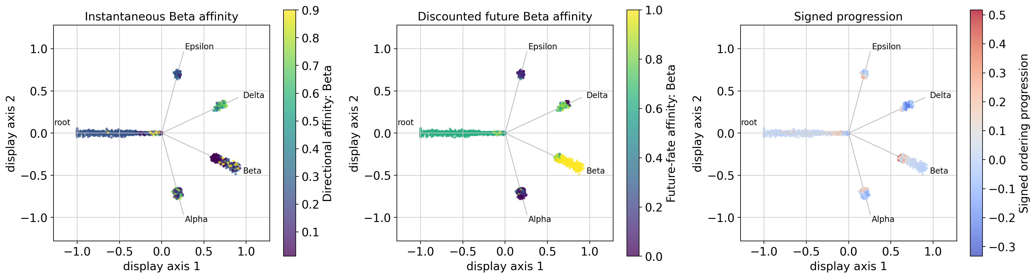
instantaneous = instantaneous_display_result
fig, axes = plt.subplots(1, 3, figsize=(18, 5))
instantaneous_display_scorer.plot_star(
    instantaneous,
    color_by="affinity:Beta",
    title="Instantaneous Beta affinity",
    ax=axes[0],
)
scorer.plot_star(
    result,
    color_by="future_fate_affinity:Beta",
    title="Discounted future Beta affinity",
    ax=axes[1],
)
scorer.plot_star(
    result,
    color_by="signed_progression",
    title="Signed progression",
    cmap="coolwarm",
    ax=axes[2],
)
fig.tight_layout()
fig.savefig(OUTPUT_DIR / "instantaneous_vs_future_fate.png", dpi=200, bbox_inches="tight")
plt.show()

../_images/tutorials_01_pancreas_single_scorer_38_0.png

19. Export reproducible analysis objects¶

[20]:

result.write_to_adata(adata)
adata.write_h5ad(OUTPUT_DIR / "pancreas_sccs_future_fate.h5ad")

cell_table = adata.obs.loc[result.cell_ids].copy()
cell_table["future_fate_reach"] = result.future_fate_reach
cell_table["future_fate_specificity"] = result.future_fate_specificity
cell_table["reach_supported_specificity"] = result.reach_supported_specificity
cell_table["signed_progression"] = result.signed_progression
cell_table["unresolved_probability"] = result.unresolved_probability
for fate_index, fate in enumerate(FATES):
    cell_table[f"future_fate_affinity_{fate}"] = result.future_fate_affinity[:, fate_index]
    cell_table[f"future_fate_contribution_{fate}"] = result.future_fate_contribution[:, fate_index]
cell_table.to_csv(OUTPUT_DIR / "cell_level_future_fate_scores.csv")
print("Saved outputs to", OUTPUT_DIR.resolve())

Saved outputs to /home/emil/notebooks/08-tutorials/tutorial_outputs/pancreas_single

20. Interpretation checklist¶

Before reporting a result, verify that:

the supervised root and fates match the biological question;
the ordering is continuous and biologically coherent;
the RNA-velocity graph was estimated outside the star geometry;
future-fate affinity is stable to a reasonable horizon/anchor range;
reach, specificity, and signed progression are reported separately;
weak Delta/Epsilon sink behavior is described rather than hidden;
candidate-gene analyses are not presented as causal evidence.