scCS Tutorial — Single-Condition Analysis
Single-cell Commitment Scores with Radial Star Embedding
scCS v0.7.0 computes RNA velocity-based commitment scores for k-furcation cell fate decisions.
What scCS does
Takes a user-defined bifurcation cluster (progenitor) and k terminal fate clusters
Builds a radial star embedding — progenitor at origin, each fate on its own arm
Projects RNA velocity into this embedding
Computes commitment scores (unCS, nCS) and per-cell fate affinities
Optionally bootstraps confidence intervals on all scores
Identifies driver genes (velocity-based + DEG-based) per fate arm
Runs pathway enrichment (KEGG, GO BP, Reactome) per fate
Reference
Kriukov et al. (2025) Single-cell transcriptome of myeloid cells in response to transplantation of human retinal neurons reveals reversibility of microglial activation
Notebook outline
Section |
What you learn |
|---|---|
|
pip install |
|
scVelo pancreas dataset |
|
scVelo dynamical model |
|
|
|
|
|
|
|
star plot, rose, pairwise heatmap, bar chart |
|
fate affinity, entropy, NN-smoothed entropy |
|
write scores back to full adata |
|
|
|
velocity drivers, DEG drivers |
|
KEGG / GO BP per fate |
|
|
1. Installation
[1]:
%matplotlib inline
# Install from GitHub (recommended)
# !pip install git+https://github.com/mcrewcow/scCS.git

# Or from a local directory:
#!pip install -e /...

import scCS
print(f"scCS version: {scCS.__version__}")
scCS version: 0.7.4
2. Load & preprocess data
We use the built-in pancreas dataset from scVelo — a well-studied k=4 bifurcation (Ductal → Alpha, Beta, Delta, Epsilon). The dataset already contains spliced/unspliced counts and cluster annotations.
[2]:
import numpy as np
import pandas as pd
import anndata
import matplotlib.pyplot as plt
import scanpy as sc
import scvelo as scv

import warnings
warnings.filterwarnings("ignore", category=DeprecationWarning)
warnings.filterwarnings("ignore", category=FutureWarning)
try:
    from statsmodels.tools.sm_exceptions import ConvergenceWarning
    warnings.filterwarnings("ignore", category=ConvergenceWarning)
except ImportError:
    pass

sc.settings.verbosity = 1
scv.settings.verbosity = 1

adata = scv.datasets.pancreas()
print(adata)
print("\nCluster labels:", adata.obs['clusters'].unique().tolist())

# --- Tutorial display helpers (compact tables instead of per-fate loops) ---
pd.set_option("display.max_rows", 20)
pd.set_option("display.max_columns", 15)
pd.set_option("display.width", 160)


def _stack_drivers(driver_dict, n_per_fate=5, cols=None):
    """Concatenate a {fate: DataFrame} dict into one tidy long-form table.

    Shows the top ``n_per_fate`` rows per fate; adds a ``fate`` column at the
    front. Pass ``cols`` to pick a subset of columns to display.
    """
    out = []
    for fate, df in driver_dict.items():
        if df is None or len(df) == 0:
            continue
        block = df.head(n_per_fate).copy()
        block.insert(0, "fate", fate)
        out.append(block)
    if not out:
        return pd.DataFrame()
    big = pd.concat(out, ignore_index=True)
    if cols is not None:
        keep = ["fate"] + [c for c in cols if c in big.columns]
        big = big[keep]
    return big


def _stack_enrichment(enrichment_dict, n_per_group=3):
    """Flatten enrichment {fate: {direction: df}} into one tidy table."""
    rows = []
    for fate, fate_results in enrichment_dict.items():
        for direction in ("up", "down"):
            df = fate_results.get(direction, None)
            if df is None or df.empty:
                continue
            top = df.head(n_per_group).copy()
            top.insert(0, "direction", direction)
            top.insert(0, "fate", fate)
            rows.append(top)
    if not rows:
        return pd.DataFrame()
    return pd.concat(rows, ignore_index=True)
AnnData object with n_obs × n_vars = 3696 × 27998
    obs: 'clusters_coarse', 'clusters', 'S_score', 'G2M_score'
    var: 'highly_variable_genes'
    uns: 'clusters_coarse_colors', 'clusters_colors', 'day_colors', 'neighbors', 'pca'
    obsm: 'X_pca', 'X_umap'
    layers: 'spliced', 'unspliced'
    obsp: 'distances', 'connectivities'

Cluster labels: ['Pre-endocrine', 'Ductal', 'Alpha', 'Ngn3 high EP', 'Delta', 'Beta', 'Ngn3 low EP', 'Epsilon']
[3]:
# Standard scVelo preprocessing
import inspect as _inspect
_fn_sig = _inspect.signature(scv.pp.filter_and_normalize).parameters
if "n_top_genes" in _fn_sig:
    scv.pp.filter_and_normalize(adata, min_shared_counts=20, n_top_genes=2000)
else:
    # scvelo builds without n_top_genes: do filter_and_normalize then HVG.
    # Use flavor="cell_ranger" not the default "seurat": seurat passes
    # int n_bins to pd.cut on log-dispersions which contain +/-inf for
    # low-mean genes — pandas >= 2.2 rejects this with ValueError.
    # cell_ranger uses explicit bin edges including +/-inf and is
    # robust across pandas/py versions (scCS changelog v0.7.4).
    scv.pp.filter_and_normalize(adata, min_shared_counts=20)
    sc.pp.highly_variable_genes(
        adata, n_top_genes=2000, subset=True, flavor="cell_ranger"
    )
sc.pp.neighbors(adata)
scv.pp.moments(adata, n_pcs=None, n_neighbors=None)
3. RNA velocity
We run the dynamical model (most accurate) via scVelo. If your data already has velocity and velocity_graph, skip this section.
[4]:
scv.tl.recover_dynamics(adata, n_jobs=32)
scv.tl.velocity(adata, mode="dynamical")
scv.tl.velocity_graph(adata)
scv.tl.velocity_pseudotime(adata)

# Visualise velocity on UMAP
scv.pl.velocity_embedding_stream(adata, basis="umap", color="clusters",
                                  title="RNA velocity — pancreas")
/home/emil/miniforge3/envs/lab-py312/lib/python3.12/multiprocessing/popen_fork.py:66: DeprecationWarning: This process (pid=3974) is multi-threaded, use of fork() may lead to deadlocks in the child.
  self.pid = os.fork()
/home/emil/miniforge3/envs/lab-py312/lib/python3.12/multiprocessing/popen_fork.py:66: DeprecationWarning: This process (pid=3974) is multi-threaded, use of fork() may lead to deadlocks in the child.
  self.pid = os.fork()
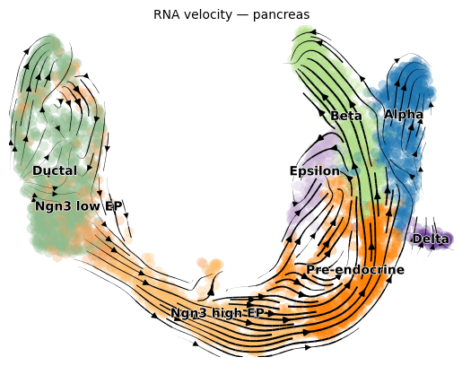
Alternatively, you can let scCS run the full velocity pipeline for you:
scorer = scCS.SingleScorer(adata, ...)
scorer.compute_velocity(mode="dynamical", n_top_genes=2000)
4. Build the radial star embedding
The pancreas dataset has a clear bifurcation from Ductal progenitors into four terminal fates: Alpha, Beta, Delta, Epsilon.
SingleScorer requires:
root— the progenitor cluster labelbranches— list of terminal fate cluster labelsobs_key— column inadata.obswith cluster labels
[5]:
scorer = scCS.SingleScorer(
    adata,
    root="Pre-endocrine",
    branches=["Alpha", "Beta", "Delta", "Epsilon"],
    obs_key="clusters",
    n_angle_bins=36,          # 10° angular bins (default)
    sector_method="centroid",  # anchor sectors to fate centroids (recommended)
)

# Build the star embedding using scVelo pseudotime
scorer.build_embedding(
    ordering_metric="pseudotime",  # uses adata.obs['velocity_pseudotime']
    arm_scale=10.0,   # maximum radial distance
    jitter=0.3,       # perpendicular noise to avoid overplotting
)

print("Embedding shape:", scorer.adata_sub.obsm["X_sccs"].shape)
print("Cells in embedding:", scorer.adata_sub.n_obs)
[scCS] Building star embedding: root='Pre-endocrine', k=4 fates, metric='pseudotime'
[scCS] Subsetting: 1876 / 3696 cells kept
       (1820 cells from other populations excluded)
       Alpha: 481 cells (fate)
       Beta: 591 cells (fate)
       Delta: 70 cells (fate)
       Epsilon: 142 cells (fate)
       Pre-endocrine: 592 cells (progenitor)

[scCS] Star embedding built → adata_sub.obsm["X_sccs"] shape: (1876, 2)
       Arm angles: {'Alpha': 0.0, 'Beta': 90.0, 'Delta': 180.0, 'Epsilon': 270.0}
[scCS] Star embedding stored in scorer.adata_sub.obsm['X_sccs']. (1876 cells)
Embedding shape: (1876, 2)
Cells in embedding: 1876
5. Fix arm coverage with subset-local pseudotime
Problem: scVelo pseudotime is computed on the full adata. When we subset to bifurcation + terminal fate cells, the pseudotime range is compressed — cells cluster near the origin instead of spanning the full arm length.
Solution: refit_pseudotime() extracts the velocity_graph submatrix for the subset cells, recomputes pseudotime locally, scales it to [0, 1], and rebuilds the embedding.
When to use ``scale_01=True`` vs ``False``:
scale_01=True(default) — cells span the full arm; best for single-condition analysis
scale_01=False— preserves absolute pseudotime ordering; use for multi-condition comparisons where cross-condition pseudotime comparability matters
[6]:
# Recompute pseudotime on the subset subgraph and rebuild the embedding
scorer.refit_pseudotime(scale_01=True)

# Inspect the corrected pseudotime
pt_sub = scorer.adata_sub.obs["velocity_pseudotime"]
print(f"Subset pseudotime range: [{pt_sub.min():.3f}, {pt_sub.max():.3f}]")
[scCS] Recomputing pseudotime on subset (1876 / 3696 cells)...
[scCS] Used scanpy DPT (with diffmap) as pseudotime fallback.
[scCS] Subset pseudotime scaled to [0, 1].
[scCS] Subset pseudotime stored in adata_sub.obs['sccs_pseudotime']. Range: [0.000, 1.000]
[scCS] Rebuilding star embedding with subset-local pseudotime...
[scCS] Subsetting: 1876 / 3696 cells kept
       (1820 cells from other populations excluded)
       Alpha: 481 cells (fate)
       Beta: 591 cells (fate)
       Delta: 70 cells (fate)
       Epsilon: 142 cells (fate)
       Pre-endocrine: 592 cells (progenitor)

[scCS] Star embedding built → adata_sub.obsm["X_sccs"] shape: (1876, 2)
       Arm angles: {'Alpha': 0.0, 'Beta': 90.0, 'Delta': 180.0, 'Epsilon': 270.0}
[scCS] Embedding rebuilt. Call fit() again to update the FateMap and velocity projection.
Subset pseudotime range: [0.495, 1.000]
6. Fit and compute commitment scores
fit() builds the FateMap (validates clusters, computes fate centroids, projects velocity). score() computes all commitment scores.
Key outputs in CommitmentScoreResult
Attribute |
Description |
|---|---|
|
Unnormalized CS matrix (k × k) |
|
Cell-count-normalized CS matrix (k × k) |
|
Fraction of velocity mass per fate |
|
Population-level commitment entropy |
|
Mean per-cell fate entropy |
|
Per-fate binary entropy |
|
Per-cell fate affinity matrix (n_cells × k) |
|
Bootstrap CI dict (if |
[7]:
scorer.fit()
[scCS] Root cluster 'Pre-endocrine': 592 cells, centroid=(-0.00, -0.00)
[scCS]   Fate 'Alpha': 481 cells, centroid=(3.51, -0.01)
[scCS]   Fate 'Beta': 591 cells, centroid=(0.03, 4.38)
[scCS]   Fate 'Delta': 70 cells, centroid=(-4.75, -0.05)
[scCS]   Fate 'Epsilon': 142 cells, centroid=(-0.02, -2.55)
[scCS] FateMap built: k=4 fates
[scCS] Projecting velocity via scVelo on full adata → slicing to subset...
[scCS] Velocity projected. Shape: (1876, 2)
FateMap  (root='Pre-endocrine', k=4)
  Cluster key : 'clusters'
  Root cells  : 592
  Root centroid: (-0.005, -0.003)
  Fate 0: 'Alpha'  n_cells=481  centroid=(3.51, -0.01)  arm_angle=0.0°
  Fate 1: 'Beta'  n_cells=591  centroid=(0.03, 4.38)  arm_angle=90.0°
  Fate 2: 'Delta'  n_cells=70  centroid=(-4.75, -0.05)  arm_angle=180.0°
  Fate 3: 'Epsilon'  n_cells=142  centroid=(-0.02, -2.55)  arm_angle=270.0°
[7]:
SingleScorer(root='Pre-endocrine', branches=['Alpha', 'Beta', 'Delta', 'Epsilon'], k=4, status='fitted')
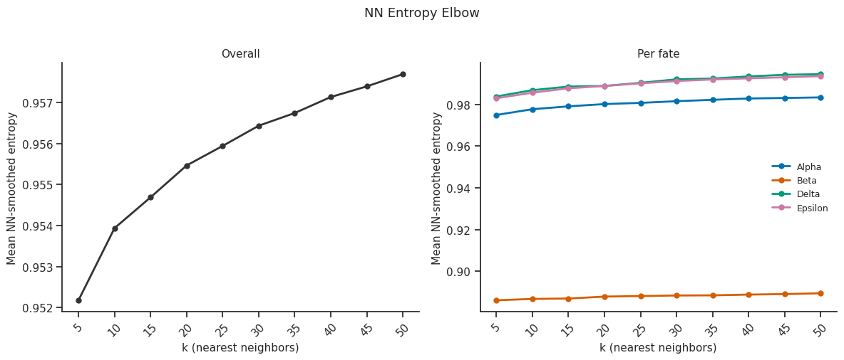
[8]:
fig = scorer.plot_nn_entropy_elbow(k_nn_range=range(5, 51, 5))
plt.show()
[9]:
# Score with bootstrap confidence intervals (n_bootstrap=500 recommended)
result = scorer.score(
    cell_level=True,   # compute per-cell fate affinities
    k_nn=15,                   # NN-smoothed entropy (15 nearest neighbours)
    n_bootstrap=500,           # bootstrap CI on nCS
    bootstrap_ci=0.95,         # 95% CI
)
[scCS] Computing bootstrap CI (n=500)...
=== CommitmentScoreResult ===
  Fates (4): Alpha, Beta, Delta, Epsilon
  Dominant fate: Beta

  Entropy metrics:
    Population entropy:           0.7052  [aggregate velocity-mass balance]
    Mean cell entropy:            0.9361  [per-cell average, k-way]
    Per-fate cell entropy:
      Alpha: 0.8246
      Beta: 0.8608
      Delta: 0.7541
      Epsilon: 0.6399
    NN-smoothed entropy (k=15):  mean=0.9547  [per-cell, stored in adata_sub.obs['cs_nn_entropy']]

  Commitment vector (normalized):
    Alpha: 0.2210
    Beta: 0.6449
    Delta: 0.0765
    Epsilon: 0.0576

  Pairwise nCS matrix:
            Alpha      Beta     Delta   Epsilon
Alpha    1.000000  0.421157  0.420532  1.133082
Beta     2.374413  1.000000  0.998516  2.690405
Delta    2.377942  1.001486  1.000000  2.694404
Epsilon  0.882548  0.371691  0.371140  1.000000

  Bootstrap 95% CI on nCS (n=500):
    CI low:
         Alpha   Beta  Delta  Epsilon
Alpha    1.000  0.369  0.352    0.922
Beta     2.119  1.000  0.851    2.270
Delta    1.989  0.855  1.000    2.103
Epsilon  0.723  0.303  0.290    1.000
    CI high:
         Alpha   Beta  Delta  Epsilon
Alpha    1.000  0.472  0.503    1.383
Beta     2.712  1.000  1.170    3.297
Delta    2.838  1.175  1.000    3.449
Epsilon  1.084  0.440  0.476    1.000
[10]:
# Summary table
print(result.summary())
=== CommitmentScoreResult ===
  Fates (4): Alpha, Beta, Delta, Epsilon
  Dominant fate: Beta

  Entropy metrics:
    Population entropy:           0.7052  [aggregate velocity-mass balance]
    Mean cell entropy:            0.9361  [per-cell average, k-way]
    Per-fate cell entropy:
      Alpha: 0.8246
      Beta: 0.8608
      Delta: 0.7541
      Epsilon: 0.6399
    NN-smoothed entropy (k=15):  mean=0.9547  [per-cell, stored in adata_sub.obs['cs_nn_entropy']]

  Commitment vector (normalized):
    Alpha: 0.2210
    Beta: 0.6449
    Delta: 0.0765
    Epsilon: 0.0576

  Pairwise nCS matrix:
            Alpha      Beta     Delta   Epsilon
Alpha    1.000000  0.421157  0.420532  1.133082
Beta     2.374413  1.000000  0.998516  2.690405
Delta    2.377942  1.001486  1.000000  2.694404
Epsilon  0.882548  0.371691  0.371140  1.000000

  Bootstrap 95% CI on nCS (n=500):
    CI low:
         Alpha   Beta  Delta  Epsilon
Alpha    1.000  0.369  0.352    0.922
Beta     2.119  1.000  0.851    2.270
Delta    1.989  0.855  1.000    2.103
Epsilon  0.723  0.303  0.290    1.000
    CI high:
         Alpha   Beta  Delta  Epsilon
Alpha    1.000  0.472  0.503    1.383
Beta     2.712  1.000  1.170    3.297
Delta    2.838  1.175  1.000    3.449
Epsilon  1.084  0.440  0.476    1.000
[11]:
# Access individual scores
print("Pairwise nCS matrix:")
print(pd.DataFrame(
    result.pairwise_nCS,
    index=result.fate_names,
    columns=result.fate_names
).round(3))

print("\nCommitment vector (fraction of velocity mass per fate):")
for fate, cv in zip(result.fate_names, result.commitment_vector):
    print(f"  {fate}: {cv:.3f}")

print(f"\nPopulation entropy: {result.population_entropy:.3f}")
print(f"Mean per-cell entropy: {result.mean_cell_entropy:.3f}")
Pairwise nCS matrix:
         Alpha   Beta  Delta  Epsilon
Alpha    1.000  0.421  0.421    1.133
Beta     2.374  1.000  0.999    2.690
Delta    2.378  1.001  1.000    2.694
Epsilon  0.883  0.372  0.371    1.000

Commitment vector (fraction of velocity mass per fate):
  Alpha: 0.221
  Beta: 0.645
  Delta: 0.076
  Epsilon: 0.058

Population entropy: 0.705
Mean per-cell entropy: 0.936
[12]:
# Bootstrap CI (if n_bootstrap > 0)
if result.bootstrap_ci is not None:
    ci = result.bootstrap_ci
    print(f"Bootstrap CI ({int(ci['ci_level']*100)}%, n={ci['n_bootstrap']}):")
    print("  nCS CI low:")
    print(pd.DataFrame(ci['ci_low'], index=result.fate_names, columns=result.fate_names).round(3))
    print("\n  nCS CI high:")
    print(pd.DataFrame(ci['ci_high'], index=result.fate_names, columns=result.fate_names).round(3))
Bootstrap CI (95%, n=500):
  nCS CI low:
         Alpha   Beta  Delta  Epsilon
Alpha    1.000  0.369  0.352    0.922
Beta     2.119  1.000  0.851    2.270
Delta    1.989  0.855  1.000    2.103
Epsilon  0.723  0.303  0.290    1.000

  nCS CI high:
         Alpha   Beta  Delta  Epsilon
Alpha    1.000  0.472  0.503    1.383
Beta     2.712  1.000  1.170    3.297
Delta    2.838  1.175  1.000    3.449
Epsilon  1.084  0.440  0.476    1.000
7. Visualizations
scCS provides several built-in plots. All are accessible as methods on the scorer or as standalone functions in scCS.plot.
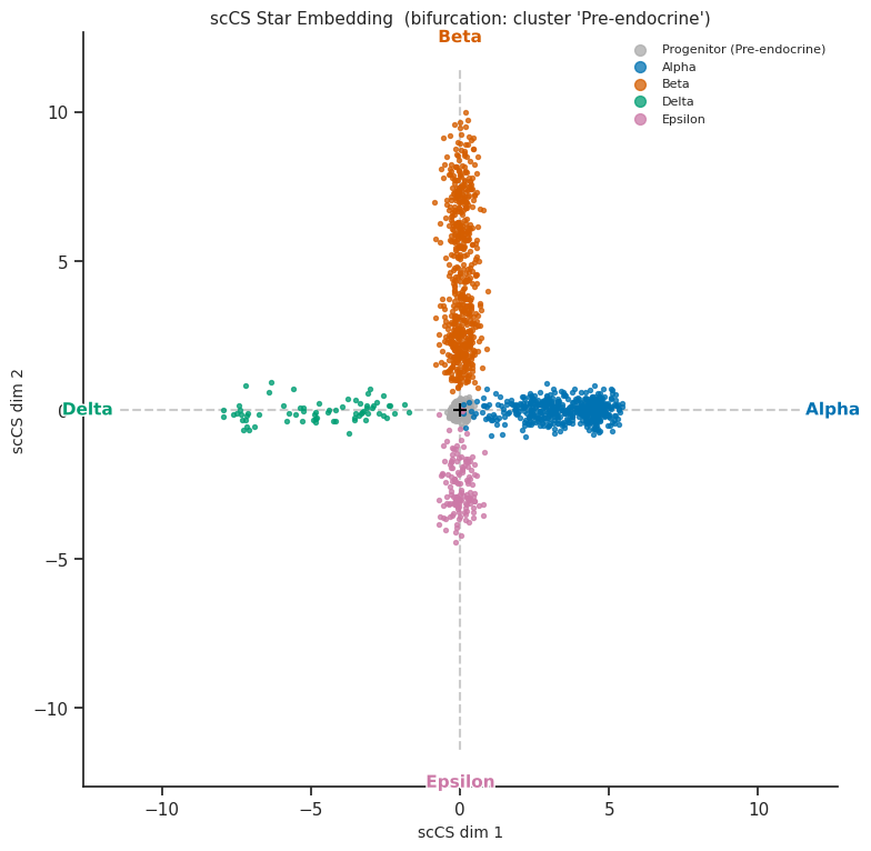
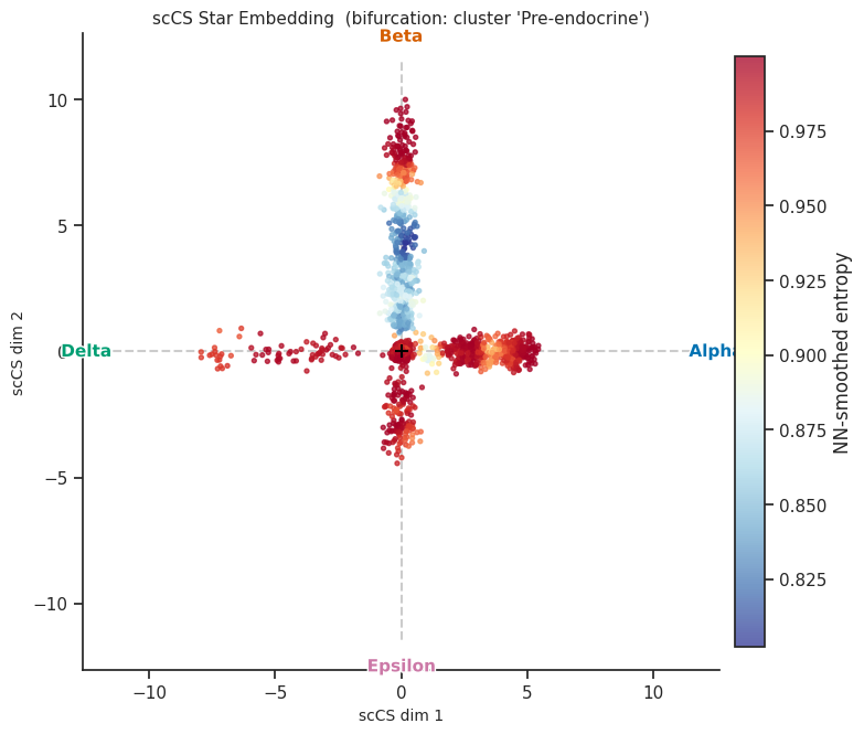
7.1 Radial star embedding
[13]:
# Primary visualization: cells in the star embedding, coloured by fate
fig = scorer.plot_star(result, figsize=(8, 8))
plt.tight_layout()
plt.show()
[14]:
# Colour by per-cell entropy instead of fate
fig = scorer.plot_star(result, color_by="entropy", figsize=(8, 8))
plt.tight_layout()
plt.show()
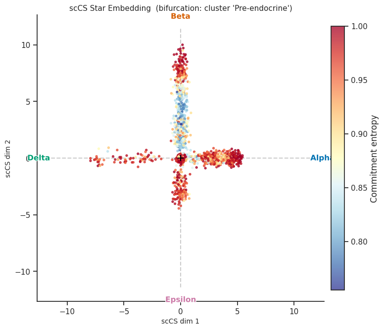
[15]:
# Colour by NN-smoothed entropy (requires k_nn in score())
fig = scorer.plot_star(result, color_by="nn_entropy", figsize=(8, 8))
plt.tight_layout()
plt.show()
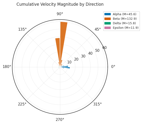
7.2 Rose / polar plot
[16]:
# Rose plot: cumulative velocity magnitude per angular bin
fig = scorer.plot_rose(result, figsize=(6, 6))
plt.tight_layout()
plt.show()
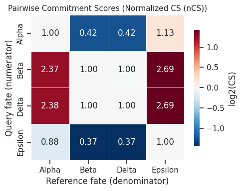
7.3 Pairwise nCS heatmap
[17]:
# Heatmap of pairwise normalized commitment scores
fig = scorer.plot_pairwise_cs(result, figsize=(5, 4))
plt.tight_layout()
plt.show()
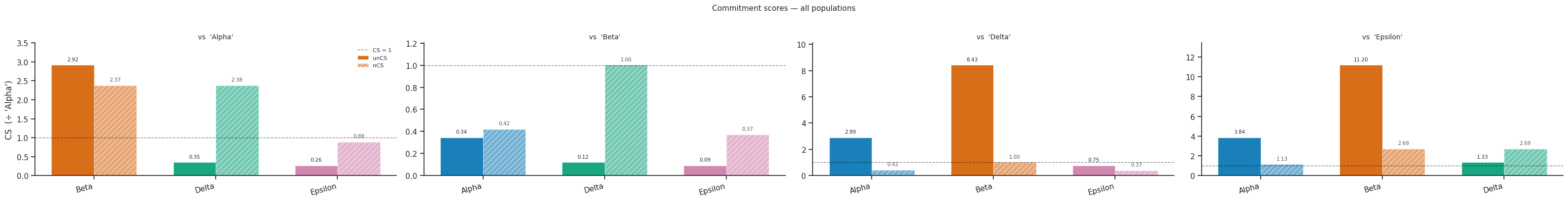
7.4 Commitment bar chart
[18]:
# Bar chart: unCS vs nCS per fate pair
fig = scorer.plot_commitment_bar(result, figsize=(8, 4))
plt.tight_layout()
plt.show()
7.5 Per-cell fate affinity heatmap
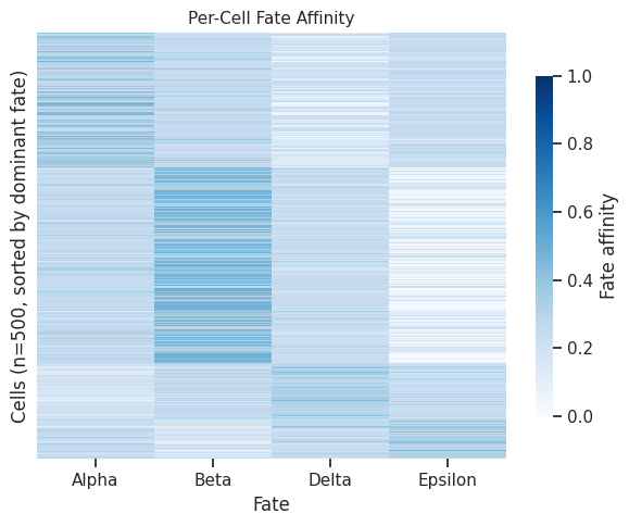
[19]:
# Heatmap of per-cell fate affinities (rows = cells, cols = fates)
fig = scorer.plot_commitment_heatmap(result, figsize=(6, 5), max_cells=500)
plt.tight_layout()
plt.show()
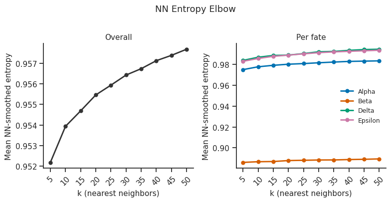
7.6 NN entropy elbow plot
[20]:
# Elbow plot to choose k_nn for NN-smoothed entropy
# Sweeps k_nn values and plots mean NN entropy
fig = scorer.plot_nn_entropy_elbow(k_nn_range=range(5, 51, 5), figsize=(8, 4))
plt.tight_layout()
plt.show()
8. Per-cell fate affinity scores
After score(cell_level=True), per-cell scores are stored in scorer.adata_sub.obs:
Column |
Description |
|---|---|
|
Per-cell affinity for each fate (sums to 1 per cell) |
|
Fate with highest affinity |
|
Per-cell commitment entropy (0 = fully committed, 1 = uniform) |
|
NN-smoothed entropy (if |
|
Subset-local pseudotime |
[21]:
# Inspect per-cell scores
obs_cols = [c for c in scorer.adata_sub.obs.columns if c.startswith("cs_")]
print("Per-cell score columns:", obs_cols)
scorer.adata_sub.obs[obs_cols].head(10)
Per-cell score columns: ['cs_Alpha', 'cs_Beta', 'cs_Delta', 'cs_Epsilon', 'cs_dominant_fate', 'cs_entropy', 'cs_nn_entropy']
[21]:
| cs_Alpha | cs_Beta | cs_Delta | cs_Epsilon | cs_dominant_fate | cs_entropy | cs_nn_entropy | |
|---|---|---|---|---|---|---|---|
| index | |||||||
| AAACCTGAGAGGGATA | 0.345656 | 0.252071 | 0.154299 | 0.247973 | Alpha | 0.972886 | 0.992053 |
| AAACCTGAGGCAATTA | 0.247055 | 0.296687 | 0.252668 | 0.203590 | Beta | 0.993692 | 0.992740 |
| AAACCTGTCCCTCTTT | 0.324502 | 0.244887 | 0.175503 | 0.255107 | Alpha | 0.983665 | 0.958981 |
| AAACGGGAGTAGCGGT | 0.361040 | 0.324278 | 0.138481 | 0.176201 | Alpha | 0.946906 | 0.977282 |
| AAACGGGCAAAGAATC | 0.274640 | 0.476842 | 0.224002 | 0.024516 | Beta | 0.818077 | 0.875318 |
| AAACGGGGTACAGTTC | 0.251495 | 0.463168 | 0.247236 | 0.038101 | Beta | 0.846585 | 0.884746 |
| AAACGGGGTCGGGTCT | 0.268075 | 0.221469 | 0.232088 | 0.278367 | Epsilon | 0.996724 | 0.998418 |
| AAACGGGTCCGCGCAA | 0.328827 | 0.381496 | 0.170364 | 0.119313 | Beta | 0.929480 | 0.988123 |
| AAACGGGTCGCATGGC | 0.272847 | 0.479499 | 0.225780 | 0.021874 | Beta | 0.812556 | 0.817800 |
| AAAGATGAGAGTACCG | 0.213046 | 0.270671 | 0.286844 | 0.229439 | Delta | 0.994829 | 0.992597 |
[22]:
# Distribution of dominant fate assignments
print(scorer.adata_sub.obs["cs_dominant_fate"].value_counts())
cs_dominant_fate
Beta       836
Alpha      604
Delta      246
Epsilon    190
Name: count, dtype: int64
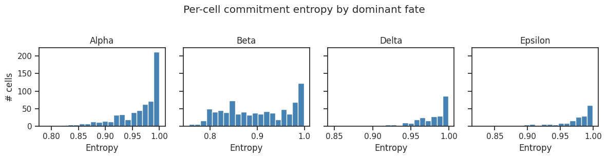
[23]:
# Entropy distribution per fate
import matplotlib.pyplot as plt

fig, axes = plt.subplots(1, len(result.fate_names), figsize=(12, 3), sharey=True)
for ax, fate in zip(axes, result.fate_names):
    mask = scorer.adata_sub.obs["cs_dominant_fate"] == fate
    ax.hist(scorer.adata_sub.obs.loc[mask, "cs_entropy"], bins=20, color="steelblue", edgecolor="white")
    ax.set_title(fate)
    ax.set_xlabel("Entropy")
axes[0].set_ylabel("# cells")
plt.suptitle("Per-cell commitment entropy by dominant fate", y=1.02)
plt.tight_layout()
plt.show()
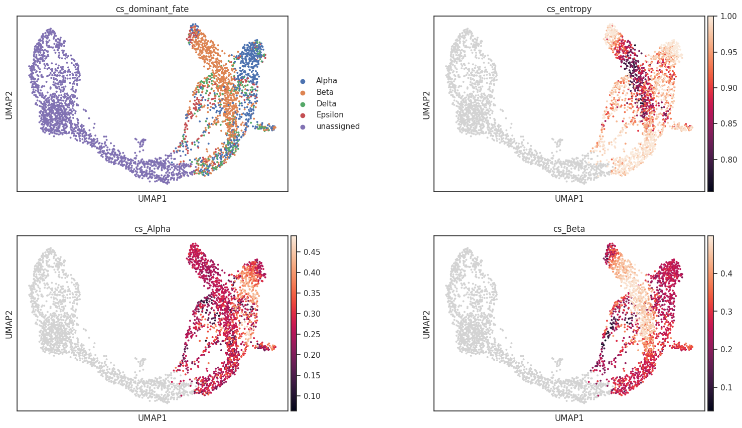
9. Transfer labels to full adata
transfer_labels() writes per-cell scores from adata_sub back to the full adata, so you can use them in UMAP plots, downstream analyses, or integration with other tools.
Cells not in the embedding subset receive NaN (numeric) or 'unassigned' (categorical).
[24]:
scorer.transfer_labels(adata, result, prefix="cs_")

# Columns added to adata.obs
cs_cols = [c for c in adata.obs.columns if c.startswith("cs_")]
print("Columns added to adata.obs:", cs_cols)
adata.obs[cs_cols].head()
[scCS] Labels transferred to adata.obs for 1876 / 3696 cells. Columns: ['cs_Alpha', 'cs_Beta', 'cs_Delta', 'cs_Epsilon', 'cs_dominant_fate', 'cs_entropy']
Columns added to adata.obs: ['cs_Alpha', 'cs_Beta', 'cs_Delta', 'cs_Epsilon', 'cs_dominant_fate', 'cs_entropy', 'cs_nn_entropy']
[24]:
| cs_Alpha | cs_Beta | cs_Delta | cs_Epsilon | cs_dominant_fate | cs_entropy | cs_nn_entropy | |
|---|---|---|---|---|---|---|---|
| index | |||||||
| AAACCTGAGAGGGATA | 0.345656 | 0.252071 | 0.154299 | 0.247973 | Alpha | 0.972886 | 0.992053 |
| AAACCTGAGCCTTGAT | NaN | NaN | NaN | NaN | unassigned | NaN | NaN |
| AAACCTGAGGCAATTA | 0.247055 | 0.296687 | 0.252668 | 0.203590 | Beta | 0.993692 | 0.992740 |
| AAACCTGCATCATCCC | NaN | NaN | NaN | NaN | unassigned | NaN | NaN |
| AAACCTGGTAAGTGGC | NaN | NaN | NaN | NaN | unassigned | NaN | NaN |
[25]:
# Visualize on UMAP
sc.pl.umap(adata, color=["cs_dominant_fate", "cs_entropy", "cs_Alpha", "cs_Beta"],
           ncols=2, wspace=0.4)
10. Subset scoring
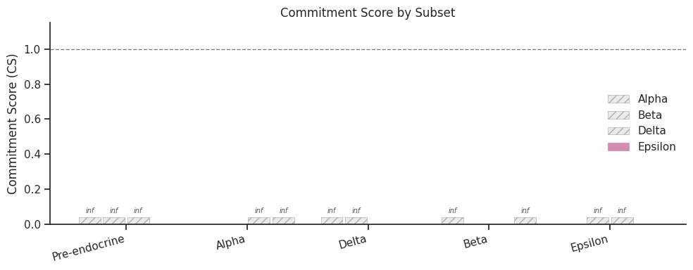
score_per_subset() computes commitment scores separately for each value of a metadata column in adata_sub.obs. Useful for comparing commitment across time points, batches, or any categorical variable.
Note: The mask is applied to
adata_sub(the embedding subset), not the full adata.
Note on ``inf`` in pairwise nCS: When a subset contains only progenitor cells (e.g., ‘Pre-endocrine’) with no cells from any fate arm,
pairwise_nCSwill beinffor all off-diagonal entries. This is mathematically correct — nCS is undefined when a fate arm has 0 cells. AUserWarningis emitted automatically. Progenitor-only subsets are still useful for inspecting the commitment vector and population entropy.
[26]:
# Score separately for each cluster within the embedding
# (Here we use 'clusters' as a demo; in practice use a condition/batch column)
subset_results = scorer.score_per_subset(
    split_by="clusters",
    cell_level=False,
    n_bootstrap=0,
    verbose=False,
)

# Tidy summary: one row per subset with all off-diagonal nCS values + status
def _subset_summary(subset_results):
    rows = []
    for subset_name, res in subset_results.items():
        n = len(res.fate_names)
        ncs = res.pairwise_nCS
        row = {"subset": subset_name, "n_cells_in_fate": int(res.n_cells_per_fate.sum())}
        for i in range(n):
            for j in range(i + 1, n):
                col = f"nCS[{res.fate_names[i]} vs {res.fate_names[j]}]"
                row[col] = float(ncs[i, j])
        # Status flag: any inf?
        off_diag = [ncs[i, j] for i in range(n) for j in range(n) if i != j]
        if all(np.isinf(v) for v in off_diag):
            row["status"] = "progenitor-only (inf)"
        elif any(np.isinf(v) for v in off_diag):
            row["status"] = "partial (some inf)"
        else:
            row["status"] = "ok"
        rows.append(row)
    return pd.DataFrame(rows)

summary_df = _subset_summary(subset_results)
summary_df
[26]:
| subset | n_cells_in_fate | nCS[Alpha vs Beta] | nCS[Alpha vs Delta] | nCS[Alpha vs Epsilon] | nCS[Beta vs Delta] | nCS[Beta vs Epsilon] | nCS[Delta vs Epsilon] | status | |
|---|---|---|---|---|---|---|---|---|---|
| 0 | Pre-endocrine | 0 | inf | inf | inf | inf | inf | inf | progenitor-only (inf) |
| 1 | Alpha | 481 | 0.0 | 0.0 | 0.0 | inf | inf | inf | partial (some inf) |
| 2 | Delta | 70 | inf | inf | inf | inf | inf | 0.0 | partial (some inf) |
| 3 | Beta | 591 | inf | inf | inf | 0.0 | 0.0 | inf | partial (some inf) |
| 4 | Epsilon | 142 | inf | inf | inf | inf | inf | inf | partial (some inf) |
[27]:
# Visualize subset comparison
fig = scorer.plot_subset_comparison(subset_results, figsize=(10, 4))
plt.tight_layout()
plt.show()
11. Driver genes
scCS provides three complementary approaches to identify fate-driving genes:
Velocity drivers (
get_velocity_drivers) — genes with highest mean RNA velocity in each fate arm (high positive velocity = gene is being upregulated along that fate)DEG drivers — differentially expressed genes between each fate arm and the bifurcation cluster (Wilcoxon rank-sum test)
Velocity-fate correlation drivers (
get_velocity_fate_drivers) — Spearman correlation between each gene’s velocity and per-cell fate affinity. Stronger signal than mean velocity because it filters out genes that are fast everywhere.
[28]:
# Velocity-based driver genes (top 20 per fate)
vel_drivers = scorer.get_velocity_drivers(n_top_genes=20)

# Compact long-form table: top 5 per fate, one DataFrame
print("Top velocity drivers (top 5 per fate):")
_stack_drivers(vel_drivers, n_per_fate=5, cols=["gene", "mean_velocity", "rank"])
── Velocity drivers: Alpha (top 20, sorted by delta_velocity) ──
 rank     gene  delta_velocity  mean_velocity
    1      Clu        1.488299       1.532060
    2     Cpa2        1.242302       0.851096
    3   Cryba2        1.057625       1.217162
    4     Ghrl        0.986426       0.384223
    5    Meis2        0.821635       0.665699
    6     Pax6        0.726139       0.883325
    7   Npepl1        0.725493       0.182687
    8   Tm4sf4        0.668253       0.466062
    9     Vasp        0.611339       0.097546
   10     Pax4        0.603224       0.034867
   11   Btbd17        0.577881       0.930656
   12     Krt7        0.547158      -0.280244
   13    Cd200        0.535196       0.330072
   14    Celf3        0.534336       0.370460
   15     Tox3        0.497146       0.251629
   16     Pdx1        0.496890       0.392475
   17   Ppp3ca        0.487356       0.200745
   18      Hn1        0.468364       0.031799
   19 BC023829        0.455840       0.336861
   20     Cpt2        0.432719       0.246379

── Velocity drivers: Beta (top 20, sorted by delta_velocity) ──
 rank          gene  delta_velocity  mean_velocity
    1          Ins2        3.672153       3.689225
    2          Nnat        3.631306       4.051527
    3          Isl1        3.562601       1.070217
    4           Clu        1.605093       1.648854
    5 1700086L19Rik        1.411600       0.453118
    6          Krt7        1.125878       0.298475
    7          Pax4        0.901425       0.333068
    8       Ppp1r1a        0.861976       1.539815
    9        Tm4sf4        0.842035       0.639844
   10       Igfbpl1        0.771356       0.268164
   11          Cpa2        0.714384       0.323178
   12          Pax6        0.697922       0.855108
   13          Dbn1        0.615245       0.314196
   14          Pdx1        0.535203       0.430788
   15         Meis2        0.518604       0.362668
   16      BC023829        0.514133       0.395154
   17         Cldn6        0.508870      -0.301879
   18         Glud1        0.481521       0.737995
   19       Smarcd2        0.460625       0.598269
   20       Lurap1l        0.456940       0.285098

── Velocity drivers: Delta (top 20, sorted by delta_velocity) ──
 rank     gene  delta_velocity  mean_velocity
    1     Cpa2        2.483908       2.092702
    2     Krt8        2.349361       1.407045
    3   Maged2        2.340670       3.380898
    4   Cryba2        1.744062       1.903599
    5     Ldha        1.710826       1.581080
    6      Hn1        1.123444       0.686879
    7   Cdkn1c        1.072009       1.007896
    8     Nnat        1.059840       1.480061
    9  Ppp1r1a        1.017116       1.694955
   10     Ambp        0.908994       0.752210
   11     Gnas        0.861592       6.604826
   12     Pax6        0.851152       1.008338
   13  Akr1c19        0.804932       1.123999
   14    Sparc        0.687036       0.649847
   15    Meis2        0.684853       0.528917
   16    Rpl12        0.670421      -0.154604
   17    Celf3        0.637237       0.473361
   18 BC023829        0.635596       0.516617
   19    Krt18        0.603725      -0.206350
   20    Foxa3        0.588107       0.411777

── Velocity drivers: Epsilon (top 20, sorted by delta_velocity) ──
 rank     gene  delta_velocity  mean_velocity
    1     Cpa2        1.345101       0.953895
    2   Cryba2        1.310028       1.469565
    3      Clu        1.293649       1.337410
    4    Meis2        1.209729       1.053792
    5     Pax4        0.843907       0.275551
    6    Syt13        0.799221       0.825314
    7    Siva1        0.731447       0.615843
    8     Pax6        0.731163       0.888349
    9  Lurap1l        0.654209       0.482367
   10  Arl6ip1        0.602216      -0.050500
   11   Nudt19        0.557069       0.466408
   12   Npepl1        0.499464      -0.043343
   13     Pdx1        0.488036       0.383621
   14    Rgs17        0.487121       0.559517
   15     Gars        0.450410       0.620145
   16     Cpt2        0.450140       0.263800
   17   Cdkn1c        0.401330       0.337217
   18 Ppp1r14b        0.393609      -0.294763
   19     Cdk1        0.393504       0.399177
   20      Tkt        0.385895       0.397531
Top velocity drivers (top 5 per fate):
[28]:
| fate | gene | mean_velocity | rank | |
|---|---|---|---|---|
| 0 | Alpha | Clu | 1.532060 | 1 |
| 1 | Alpha | Cpa2 | 0.851096 | 2 |
| 2 | Alpha | Cryba2 | 1.217162 | 3 |
| 3 | Alpha | Ghrl | 0.384223 | 4 |
| 4 | Alpha | Meis2 | 0.665699 | 5 |
| 5 | Beta | Ins2 | 3.689225 | 1 |
| 6 | Beta | Nnat | 4.051527 | 2 |
| 7 | Beta | Isl1 | 1.070217 | 3 |
| 8 | Beta | Clu | 1.648854 | 4 |
| 9 | Beta | 1700086L19Rik | 0.453118 | 5 |
| 10 | Delta | Cpa2 | 2.092702 | 1 |
| 11 | Delta | Krt8 | 1.407045 | 2 |
| 12 | Delta | Maged2 | 3.380898 | 3 |
| 13 | Delta | Cryba2 | 1.903599 | 4 |
| 14 | Delta | Ldha | 1.581080 | 5 |
| 15 | Epsilon | Cpa2 | 0.953895 | 1 |
| 16 | Epsilon | Cryba2 | 1.469565 | 2 |
| 17 | Epsilon | Clu | 1.337410 | 3 |
| 18 | Epsilon | Meis2 | 1.053792 | 4 |
| 19 | Epsilon | Pax4 | 0.275551 | 5 |
[29]:
# DEG-based driver genes (top 20 per fate, vs the bifurcation cluster)
deg_drivers = scorer.get_deg_drivers(
    n_top_genes=20,
    pval_threshold=0.05,
    logfc_threshold=0.25,
)

print("Top DEG drivers (top 5 per fate):")
_stack_drivers(
    deg_drivers, n_per_fate=5,
    cols=["gene", "logfoldchange", "pval_adj", "pct_fate", "pct_progenitor"],
)
── DEG drivers: Alpha vs progenitor ──
   Significant: 761  (up: 376, down: 385)
   gene  logfoldchange      pval_adj  pct_fate  pct_progenitor
    Pyy     209.768677  1.181761e-93  0.968815             NaN
    Gcg     209.614731  9.196179e-64  0.656965             NaN
   Iapp      99.370232  4.065913e-99  0.854470             NaN
    Ttr      67.718864 2.617159e-103  1.000000             NaN
   Gnas      34.805965  2.937512e-52  1.000000             NaN
   Rbp4      33.815922  7.031753e-50  0.962578             NaN
  Hpgds      26.723766  3.763407e-02  0.087318             NaN
    Tnr      26.722797  2.795890e-02  0.091476             NaN
 Tmem27      17.364475 1.123328e-141  0.981289             NaN
Slc38a5      15.393972  4.940813e-60  0.920998             NaN
 Pcsk1n      12.127839  4.762578e-59  0.997921             NaN
   Gast       9.842274  1.419605e-32  0.538462             NaN
    Cpe       7.672148  1.079724e-40  1.000000             NaN
  Pcsk2       7.646369  6.491126e-63  0.846154             NaN
   Gpx3       7.507235  1.191563e-82  0.937630             NaN
  Meis2       6.603501  2.217035e-78  0.970894             NaN
  Peg10       6.532975  2.869438e-65  0.700624             NaN
   Ssr2       6.296807  1.585608e-69  0.985447             NaN
    Ppy       6.134921  1.251811e-15  0.378378             NaN
Tmsb15l       5.803368  2.070066e-73  0.711019             NaN

── DEG drivers: Beta vs progenitor ──
   Significant: 830  (up: 422, down: 408)
   gene  logfoldchange      pval_adj  pct_fate  pct_progenitor
   Iapp     185.345184 6.106240e-152  0.944162             NaN
    Pyy     139.123322  1.052978e-85  0.962775             NaN
   Ins1      99.108521  3.512617e-47  0.582064             NaN
   Ins2      47.560135  3.515790e-67  0.610829             NaN
   Nnat      42.420864 2.029962e-103  0.825719             NaN
   Rbp4      41.067871 6.750219e-103  0.996616             NaN
  P2ry1      27.845049  4.690784e-06  0.164129             NaN
   Fmo1      26.452681  3.894453e-02  0.081218             NaN
 Plppr1      26.415466  3.894453e-02  0.081218             NaN
   Gnas      26.366089  3.362044e-60  1.000000             NaN
    Ttr      22.955372  6.047775e-52  0.994924             NaN
   Dlk1      12.507628  4.599450e-97  0.966159             NaN
 Sec61b      12.047029 6.698179e-114  1.000000             NaN
    Npy      12.042974  1.086211e-07  0.191201             NaN
Ppp1r1a      11.322408  1.013795e-94  0.712352             NaN
  Pcsk2       9.181964 2.013853e-127  0.984772             NaN
   Calr       8.696516  3.976336e-95  0.959391             NaN
  Rpl10       8.650661  6.788600e-35  1.000000             NaN
  Hspa5       8.530251 2.027799e-109  0.969543             NaN
 Sdf2l1       7.616785  3.683485e-85  0.747885             NaN

── DEG drivers: Delta vs progenitor ──
   Significant: 386  (up: 156, down: 230)
  gene  logfoldchange     pval_adj  pct_fate  pct_progenitor
   Pyy     484.160583 5.419924e-34  1.000000             NaN
   Sst     332.010773 9.905999e-30  0.871429             NaN
  Rbp4     194.580841 2.024127e-37  1.000000             NaN
  Iapp     102.586014 2.319858e-35  0.985714             NaN
Ptprz1      28.902637 3.369656e-03  0.257143             NaN
 Cd24a      20.200207 1.633998e-31  1.000000             NaN
   Ppy      18.444256 6.494096e-07  0.485714             NaN
  Hhex      16.970627 6.566081e-31  0.985714             NaN
  Dlk1      16.967428 4.469675e-28  1.000000             NaN
 Rpl10      13.510839 4.188939e-13  1.000000             NaN
  Ssr2      10.061992 2.442933e-24  1.000000             NaN
  Gpx3       9.890513 3.689698e-25  0.985714             NaN
  Isl1       9.400220 3.580594e-12  1.000000             NaN
  Hadh       9.289947 7.724100e-31  0.971429             NaN
  Arg1       8.830122 9.905999e-30  0.900000             NaN
 Pcsk2       8.306222 1.427407e-20  0.928571             NaN
   Ttr       7.740336 4.406957e-03  0.971429             NaN
Spock3       7.235566 4.338918e-05  0.342857             NaN
  Mest       6.525658 6.399791e-18  0.714286             NaN
Igfbp7       6.383225 4.517170e-17  0.685714             NaN

── DEG drivers: Epsilon vs progenitor ──
   Significant: 518  (up: 266, down: 252)
   gene  logfoldchange     pval_adj  pct_fate  pct_progenitor
   Ghrl     495.486511 3.376669e-72  1.000000             NaN
    Pyy      81.501137 3.980708e-18  0.873239             NaN
   Rbp4      74.675728 6.843394e-44  0.992958             NaN
 Lrpprc      22.582724 8.565872e-16  0.873239             NaN
 Cdkn1a      21.258612 4.533111e-15  0.887324             NaN
    Gcg      20.178659 1.772858e-04  0.338028             NaN
   Iapp      18.956543 1.029570e-23  0.760563             NaN
   Isl1      18.905531 3.368229e-35  0.992958             NaN
    Ttr      16.562450 4.734949e-04  0.929577             NaN
 Maged2      15.220592 1.711104e-41  0.943662             NaN
  Hspa5       9.455750 8.303204e-39  0.957746             NaN
 Tmem27       8.894045 2.939794e-24  0.739437             NaN
   Calr       8.733923 2.532672e-39  0.950704             NaN
   Ssr2       7.860883 2.188520e-39  0.992958             NaN
   Arg1       7.192320 3.382770e-34  0.732394             NaN
  Rpl10       7.168509 2.855208e-09  1.000000             NaN
Slc38a5       7.034479 3.542731e-11  0.838028             NaN
  Ccnd2       6.007015 4.025146e-26  0.661972             NaN
  Acsl1       5.986801 1.903084e-05  0.267606             NaN
  Anpep       5.644922 5.435417e-36  0.802817             NaN
Top DEG drivers (top 5 per fate):
[29]:
| fate | gene | logfoldchange | pval_adj | pct_fate | pct_progenitor | |
|---|---|---|---|---|---|---|
| 0 | Alpha | Pyy | 209.768677 | 1.181761e-93 | 0.968815 | NaN |
| 1 | Alpha | Gcg | 209.614731 | 9.196179e-64 | 0.656965 | NaN |
| 2 | Alpha | Iapp | 99.370232 | 4.065913e-99 | 0.854470 | NaN |
| 3 | Alpha | Ttr | 67.718864 | 2.617159e-103 | 1.000000 | NaN |
| 4 | Alpha | Gnas | 34.805965 | 2.937512e-52 | 1.000000 | NaN |
| 5 | Beta | Iapp | 185.345184 | 6.106240e-152 | 0.944162 | NaN |
| 6 | Beta | Pyy | 139.123322 | 1.052978e-85 | 0.962775 | NaN |
| 7 | Beta | Ins1 | 99.108521 | 3.512617e-47 | 0.582064 | NaN |
| 8 | Beta | Ins2 | 47.560135 | 3.515790e-67 | 0.610829 | NaN |
| 9 | Beta | Nnat | 42.420864 | 2.029962e-103 | 0.825719 | NaN |
| 10 | Delta | Pyy | 484.160583 | 5.419924e-34 | 1.000000 | NaN |
| 11 | Delta | Sst | 332.010773 | 9.905999e-30 | 0.871429 | NaN |
| 12 | Delta | Rbp4 | 194.580841 | 2.024127e-37 | 1.000000 | NaN |
| 13 | Delta | Iapp | 102.586014 | 2.319858e-35 | 0.985714 | NaN |
| 14 | Delta | Ptprz1 | 28.902637 | 3.369656e-03 | 0.257143 | NaN |
| 15 | Epsilon | Ghrl | 495.486511 | 3.376669e-72 | 1.000000 | NaN |
| 16 | Epsilon | Pyy | 81.501137 | 3.980708e-18 | 0.873239 | NaN |
| 17 | Epsilon | Rbp4 | 74.675728 | 6.843394e-44 | 0.992958 | NaN |
| 18 | Epsilon | Tnr | 26.569187 | 2.522357e-01 | 0.091549 | NaN |
| 19 | Epsilon | Hpgds | 26.106819 | 4.514074e-01 | 0.070423 | NaN |
11.3 Velocity-fate correlation drivers
get_velocity_fate_drivers() computes the Spearman correlation between each gene’s velocity and the per-cell fate affinity score for each fate arm. Genes with high positive correlation are being upregulated specifically as cells commit to that fate — a stronger signal than mean velocity alone, because it filters out genes that are fast everywhere.
Requires score(cell_level=True) to have been called first (needs result.cell_scores).
[30]:
# Velocity-fate correlation drivers
# Correlates each gene's velocity with per-cell fate affinity scores
# (requires cell_level=True in score())
try:
    vf_drivers = scorer.get_velocity_fate_drivers(
        result,
        n_top_genes=20,
        pval_threshold=0.05,
    )
    print("Top velocity-fate drivers (top 5 per fate):")
    display(_stack_drivers(
        vf_drivers, n_per_fate=5,
        cols=["gene", "spearman_r", "pval_adj", "mean_velocity", "delta_velocity"],
    ))
except ValueError as e:
    print(f"Skipped: {e}")
    print("Tip: call scorer.score(cell_level=True) first.")
── Velocity-fate drivers: Alpha (top 20, sorted by Spearman r) ──
   Significant (FDR < 0.05): 683 / 2000
 rank          gene  spearman_r     pval_adj  mean_velocity
    1        Adam23    0.332275 2.726568e-46       0.035280
    2           Klb    0.309560 6.025260e-40       0.045717
    3       Tmem206    0.265787 4.237692e-29       0.099139
    4        Notch2    0.257026 2.741812e-27       0.073804
    5        Sorcs2    0.235934 5.877863e-23       0.037468
    6       Rasgrf2    0.235511 6.661376e-23       0.025164
    7         Epha4    0.235026 7.813431e-23       0.052760
    8        Megf11    0.228079 1.824037e-21       0.007886
    9          Sgce    0.224234 9.184396e-21       0.052389
   10         Kif2c    0.223713 1.097454e-20       0.083291
   11         Sel1l    0.223152 1.274883e-20       0.055911
   12          Bst2    0.222681 1.434448e-20       0.190410
   13          Ctsb    0.219757 4.981190e-20      -0.068126
   14        Gabrb3    0.217725 1.071893e-19       0.055429
   15        Tmem51    0.214352 4.378911e-19       0.109053
   16       Fam234a    0.214279 4.378911e-19       0.044228
   17 1700011H14Rik    0.212987 7.086263e-19       0.285092
   18          Gch1    0.211215 1.369510e-18       0.472799
   19         Cdh11    0.211206 1.369510e-18       0.021027
   20       Zcchc16    0.210129 2.081817e-18       0.022147

── Velocity-fate drivers: Beta (top 20, sorted by Spearman r) ──
   Significant (FDR < 0.05): 924 / 2000
 rank    gene  spearman_r      pval_adj  mean_velocity
    1   Gng12    0.687204 4.410440e-259       0.364720
    2    Nnat    0.675808 1.430221e-247       4.051527
    3    Sdk2    0.571355 3.286960e-160       0.011898
    4   Dact2    0.559535 2.499373e-152       0.045325
    5   Ap1s2    0.549641 5.731258e-146       0.087439
    6   Vat1l    0.548981 1.264673e-145       0.064852
    7  Sphkap    0.541680 4.498258e-141       0.119721
    8    Mxd4    0.515216 2.594995e-125      -0.069785
    9  Slc2a2    0.511380 2.850628e-123       0.166863
   10    Nol4    0.506439 1.524017e-120       0.096487
   11 Shroom3    0.501075 1.259699e-117      -0.008355
   12  Zbtb7c    0.497687 7.505370e-116       0.024958
   13    Ins2    0.488525 5.173891e-111       3.689225
   14 Igfbpl1    0.474913 3.992365e-104       0.268164
   15 Slc7a14    0.461875  7.903311e-98       0.072172
   16  Ptprz1    0.459658  8.304841e-97       0.021035
   17   Ccnd2    0.458424  3.072975e-96       0.365967
   18      Gc    0.455471  7.272239e-95       0.137919
   19     Ghr    0.454304  2.464647e-94       0.248989
   20 Slc30a8    0.449188  5.200257e-92       0.450795

── Velocity-fate drivers: Delta (top 20, sorted by Spearman r) ──
   Significant (FDR < 0.05): 685 / 2000
 rank     gene  spearman_r     pval_adj  mean_velocity
    1   Zbtb20    0.303609 1.783641e-38       0.166360
    2   Fndc3a    0.293026 9.165943e-36      -0.005701
    3    Pbld2    0.258827 1.428849e-27       0.038566
    4    Vat1l    0.252901 2.293744e-26       0.065950
    5   Trim35    0.250792 5.950762e-26       0.184455
    6     Hap1    0.248696 1.537300e-25       0.031227
    7      Arx    0.245404 7.175120e-25      -0.018569
    8     Asb4    0.236969 3.565400e-23      -0.003783
    9   Vps37a    0.227608 2.126823e-21      -0.083059
   10     Chd3    0.223959 9.343843e-21      -0.079594
   11   Snap25    0.222951 1.330732e-20       0.048876
   12     Mia3    0.221878 2.046525e-20       0.047561
   13     Ufm1    0.217722 1.073379e-19      -0.142988
   14  Stard10    0.214950 3.289204e-19      -0.088858
   15 BC048546    0.214442 3.949377e-19      -0.140049
   16     Pon2    0.208136 4.756439e-18      -0.013737
   17     Tmx1    0.203896 2.536844e-17      -0.220162
   18      Cpm    0.202291 4.706904e-17       0.038128
   19     Gcsh    0.201279 6.868679e-17      -0.086339
   20     Hagh    0.198569 1.954275e-16       0.038047

── Velocity-fate drivers: Epsilon (top 20, sorted by Spearman r) ──
   Significant (FDR < 0.05): 924 / 2000
 rank    gene  spearman_r      pval_adj  mean_velocity
    1  Rab27a    0.514252 8.184805e-125       0.055813
    2    Pdk2    0.512925 4.186366e-124       0.051594
    3  Sorcs1    0.499450 8.951898e-117       0.005206
    4  Il17re    0.485971 1.042002e-109      -0.002558
    5   Auts2    0.484087 9.271443e-109       0.256760
    6   Pycr2    0.474232 8.299458e-104      -0.452137
    7  Nusap1    0.467321 2.024908e-100       0.014434
    8    Mnx1    0.465603  1.321285e-99      -0.004751
    9    Chga    0.460968  2.055227e-97      -2.422998
   10  Npepl1    0.449508  3.960569e-92      -0.043343
   11   Gm609    0.449416  4.222258e-92       0.024659
   12 Efcab10    0.448844  7.240713e-92      -0.045064
   13   Gsto1    0.445875  1.588429e-90      -0.086271
   14   Igf1r    0.445424  2.468092e-90      -0.019749
   15  Eps8l2    0.442219  6.679705e-89       0.126253
   16   Kcnb2    0.441447  1.439386e-88       0.029580
   17 Cbfa2t2    0.432747  9.568963e-85       0.159800
   18 Fam213a    0.432126  1.687532e-84       0.043521
   19   Josd2    0.428882  4.017044e-83       0.046612
   20  Kif20a    0.428003  9.327305e-83       0.081612
Top velocity-fate drivers (top 5 per fate):
| fate | gene | spearman_r | pval_adj | mean_velocity | delta_velocity | |
|---|---|---|---|---|---|---|
| 0 | Alpha | Adam23 | 0.332275 | 2.726568e-46 | 0.035280 | 0.026601 |
| 1 | Alpha | Klb | 0.309560 | 6.025260e-40 | 0.045717 | 0.037019 |
| 2 | Alpha | Tmem206 | 0.265787 | 4.237692e-29 | 0.099139 | 0.149552 |
| 3 | Alpha | Notch2 | 0.257026 | 2.741812e-27 | 0.073804 | 0.069658 |
| 4 | Alpha | Sorcs2 | 0.235934 | 5.877863e-23 | 0.037468 | 0.026698 |
| 5 | Beta | Gng12 | 0.687204 | 4.410440e-259 | 0.364720 | 0.065286 |
| 6 | Beta | Nnat | 0.675808 | 1.430221e-247 | 4.051527 | 3.631306 |
| 7 | Beta | Sdk2 | 0.571355 | 3.286960e-160 | 0.011898 | 0.011638 |
| 8 | Beta | Dact2 | 0.559535 | 2.499373e-152 | 0.045325 | 0.018165 |
| 9 | Beta | Ap1s2 | 0.549641 | 5.731258e-146 | 0.087439 | 0.024644 |
| 10 | Delta | Zbtb20 | 0.303609 | 1.783641e-38 | 0.166360 | -0.036171 |
| 11 | Delta | Fndc3a | 0.293026 | 9.165943e-36 | -0.005701 | -0.049914 |
| 12 | Delta | Pbld2 | 0.258827 | 1.428849e-27 | 0.038566 | 0.025424 |
| 13 | Delta | Vat1l | 0.252901 | 2.293744e-26 | 0.065950 | 0.013837 |
| 14 | Delta | Trim35 | 0.250792 | 5.950762e-26 | 0.184455 | 0.063726 |
| 15 | Epsilon | Rab27a | 0.514252 | 8.184805e-125 | 0.055813 | 0.007661 |
| 16 | Epsilon | Pdk2 | 0.512925 | 4.186366e-124 | 0.051594 | 0.072639 |
| 17 | Epsilon | Sorcs1 | 0.499450 | 8.951898e-117 | 0.005206 | 0.004127 |
| 18 | Epsilon | Il17re | 0.485971 | 1.042002e-109 | -0.002558 | -0.027604 |
| 19 | Epsilon | Auts2 | 0.484087 | 9.271443e-109 | 0.256760 | 0.302319 |
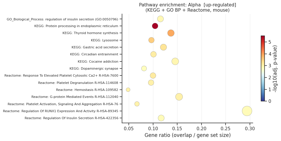
12. Pathway enrichment
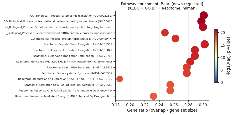
get_enrichment() runs over-representation analysis (ORA) on the DEG driver genes for each fate using gseapy (KEGG, GO Biological Process, Reactome).
Requires an internet connection and a valid organism code.
[31]:
# Pathway enrichment per fate
# Note: requires gseapy and internet access for Enrichr API
# Results will be empty with synthetic data (too few significant DEGs)

try:
    enrichment = scorer.get_enrichment(
        deg_drivers,
        organism="mouse",     # "mouse" or "human"
        pval_threshold=0.05,
        logfc_threshold=0.25,
        plot=True,            # dot plots saved per fate
        n_top_pathways=15,
    )

    # Single compact summary: top 3 pathways per (fate, direction)
    enrich_df = _stack_enrichment(enrichment, n_per_group=3)
    if not enrich_df.empty:
        display(enrich_df[["fate", "direction", "Gene_set", "Term", "Overlap", "Adjusted P-value"]])
    else:
        print("(No enriched terms — typical with small / synthetic datasets.)")

except ImportError:
    print("gseapy not installed. Run: pip install gseapy")
except Exception as e:
    print(f"Enrichment skipped: {e}")
    print("(Expected with synthetic data — use real data for meaningful results.)")
============================================================
Pathway enrichment: Alpha
Gene sets: ['KEGG_2019_Mouse', 'GO_Biological_Process_2021', 'Reactome_2022']
Up-regulated genes : 376
Down-regulated genes: 385
============================================================
[up] Significant terms: 121
Gene_set Term Overlap Adjusted P-value
KEGG_2019_Mouse Protein processing in endoplasmic reticulum 17/163 0.000003
KEGG_2019_Mouse Thyroid hormone synthesis 10/73 0.000127
KEGG_2019_Mouse Lysosome 12/124 0.000313
KEGG_2019_Mouse Gastric acid secretion 9/74 0.000600
Reactome_2022 Response To Elevated Platelet Cytosolic Ca2+ R-HSA-76005 13/130 0.000783
KEGG_2019_Mouse Circadian entrainment 10/99 0.000825
Reactome_2022 Platelet Degranulation R-HSA-114608 12/125 0.000966
Reactome_2022 Hemostasis R-HSA-109582 28/576 0.000966
Reactome_2022 G-protein Mediated Events R-HSA-112040 8/52 0.000966
Reactome_2022 Platelet Activation, Signaling And Aggregation R-HSA-76002 17/254 0.001008
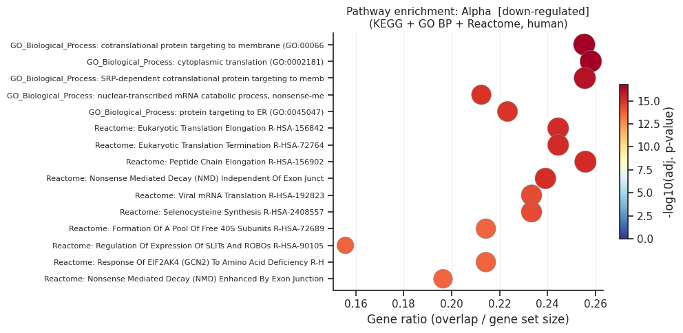
[down] Significant terms: 252
Gene_set Term Overlap Adjusted P-value
GO_Biological_Process_2021 cotranslational protein targeting to membrane (GO:0006613) 24/94 1.627570e-17
GO_Biological_Process_2021 cytoplasmic translation (GO:0002181) 24/93 1.627570e-17
GO_Biological_Process_2021 SRP-dependent cotranslational protein targeting to membrane (GO:0006614) 23/90 6.790532e-17
Reactome_2022 Eukaryotic Translation Elongation R-HSA-156842 22/90 5.465181e-16
Reactome_2022 Eukaryotic Translation Termination R-HSA-72764 22/90 5.465181e-16
Reactome_2022 Peptide Chain Elongation R-HSA-156902 22/86 5.465181e-16
Reactome_2022 Nonsense Mediated Decay (NMD) Independent Of Exon Junction Complex (EJC) R-HSA-975956 22/92 6.859847e-16
GO_Biological_Process_2021 nuclear-transcribed mRNA catabolic process, nonsense-mediated decay (GO:0000184) 24/113 8.686504e-16
GO_Biological_Process_2021 protein targeting to ER (GO:0045047) 23/103 1.101897e-15
Reactome_2022 Viral mRNA Translation R-HSA-192823 21/90 4.696474e-15
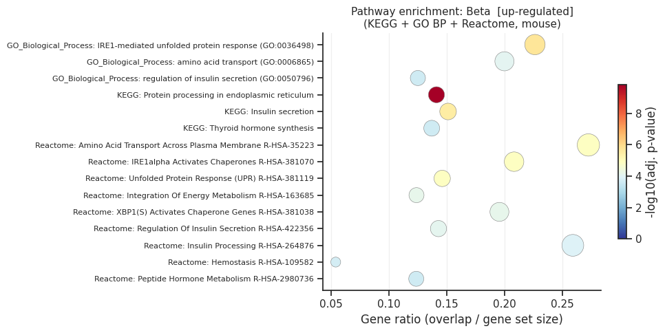
============================================================
  Pathway enrichment: Beta
  Gene sets: ['KEGG_2019_Mouse', 'GO_Biological_Process_2021', 'Reactome_2022']
  Up-regulated genes  : 422
  Down-regulated genes: 408
============================================================

  [up] Significant terms: 121
                  Gene_set                                                     Term Overlap  Adjusted P-value
           KEGG_2019_Mouse              Protein processing in endoplasmic reticulum  23/163      1.407868e-10
GO_Biological_Process_2021     IRE1-mediated unfolded protein response (GO:0036498)   12/53      1.863342e-06
           KEGG_2019_Mouse                                        Insulin secretion   13/86      3.415612e-06
             Reactome_2022 Amino Acid Transport Across Plasma Membrane R-HSA-352230    9/33      1.321921e-05
             Reactome_2022              IRE1alpha Activates Chaperones R-HSA-381070   10/48      1.321921e-05
             Reactome_2022             Unfolded Protein Response (UPR) R-HSA-381119   13/89      1.321921e-05
             Reactome_2022            Integration Of Energy Metabolism R-HSA-163685  13/105      6.483513e-05
             Reactome_2022           XBP1(S) Activates Chaperone Genes R-HSA-381038    9/46      6.628341e-05
             Reactome_2022             Regulation Of Insulin Secretion R-HSA-422356   11/77      8.152971e-05
GO_Biological_Process_2021                        amino acid transport (GO:0006865)   10/50      8.704602e-05

  [down] Significant terms: 245
                  Gene_set                                                                                  Term Overlap  Adjusted P-value
GO_Biological_Process_2021                                                  cytoplasmic translation (GO:0002181)   28/93      4.333388e-22
GO_Biological_Process_2021                            cotranslational protein targeting to membrane (GO:0006613)   28/94      4.333388e-22
GO_Biological_Process_2021              SRP-dependent cotranslational protein targeting to membrane (GO:0006614)   27/90      1.679608e-21
             Reactome_2022                                                 Peptide Chain Elongation R-HSA-156902   26/86      1.148227e-20
             Reactome_2022                                        Eukaryotic Translation Elongation R-HSA-156842   26/90      1.428872e-20
             Reactome_2022                                        Eukaryotic Translation Termination R-HSA-72764   26/90      1.428872e-20
             Reactome_2022 Nonsense Mediated Decay (NMD) Independent Of Exon Junction Complex (EJC) R-HSA-975956   26/92      2.014986e-20
GO_Biological_Process_2021      nuclear-transcribed mRNA catabolic process, nonsense-mediated decay (GO:0000184)  28/113      5.547475e-20
GO_Biological_Process_2021                                                  protein targeting to ER (GO:0045047)  27/103      5.547475e-20
             Reactome_2022                                                   Viral mRNA Translation R-HSA-192823   25/90      1.461345e-19
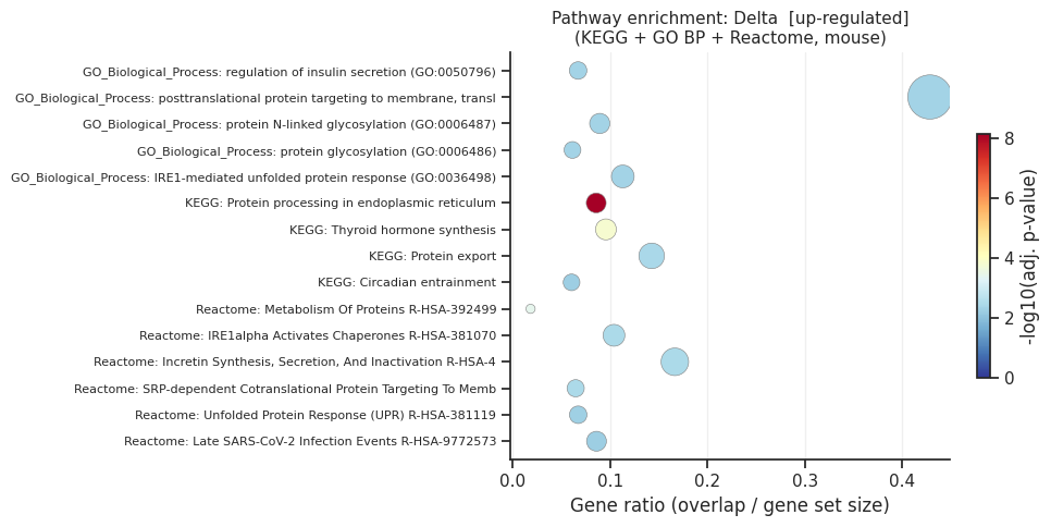
============================================================
  Pathway enrichment: Delta
  Gene sets: ['KEGG_2019_Mouse', 'GO_Biological_Process_2021', 'Reactome_2022']
  Up-regulated genes  : 156
  Down-regulated genes: 230
============================================================

  [up] Significant terms: 41
                  Gene_set                                                                        Term Overlap  Adjusted P-value
           KEGG_2019_Mouse                                 Protein processing in endoplasmic reticulum  14/163      6.690234e-09
           KEGG_2019_Mouse                                                   Thyroid hormone synthesis    7/73      1.429359e-04
             Reactome_2022                                         Metabolism Of Proteins R-HSA-392499 35/1890      3.776032e-04
             Reactome_2022                                 IRE1alpha Activates Chaperones R-HSA-381070    5/48      3.289099e-03
             Reactome_2022                Incretin Synthesis, Secretion, And Inactivation R-HSA-400508    4/24      3.289099e-03
             Reactome_2022   SRP-dependent Cotranslational Protein Targeting To Membrane R-HSA-1799339   7/108      3.289099e-03
           KEGG_2019_Mouse                                                              Protein export    4/28      3.697039e-03
GO_Biological_Process_2021                                regulation of insulin secretion (GO:0050796)   7/104      4.368748e-03
GO_Biological_Process_2021 posttranslational protein targeting to membrane, translocation (GO:0031204)     3/7      4.368748e-03
GO_Biological_Process_2021                                 protein N-linked glycosylation (GO:0006487)    6/67      4.368748e-03
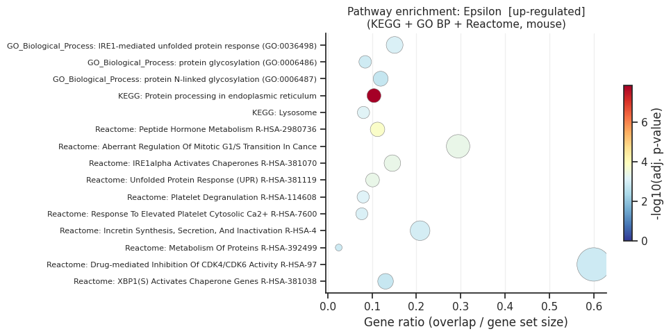
============================================================
Pathway enrichment: Epsilon
Gene sets: ['KEGG_2019_Mouse', 'GO_Biological_Process_2021', 'Reactome_2022']
Up-regulated genes : 266
Down-regulated genes: 252
============================================================
[up] Significant terms: 47
Gene_set Term Overlap Adjusted P-value
KEGG_2019_Mouse Protein processing in endoplasmic reticulum 17/163 1.392463e-08
Reactome_2022 Peptide Hormone Metabolism R-HSA-2980736 10/89 1.607304e-04
Reactome_2022 Aberrant Regulation Of Mitotic G1/S Transition In Cancer Due To RB1 Defects R-HSA-9659787 5/17 4.275598e-04
Reactome_2022 IRE1alpha Activates Chaperones R-HSA-381070 7/48 4.275598e-04
Reactome_2022 Unfolded Protein Response (UPR) R-HSA-381119 9/89 4.275598e-04
KEGG_2019_Mouse Lysosome 10/124 6.781878e-04
Reactome_2022 Platelet Degranulation R-HSA-114608 10/125 7.374527e-04
GO_Biological_Process_2021 IRE1-mediated unfolded protein response (GO:0036498) 8/53 8.563951e-04
Reactome_2022 Response To Elevated Platelet Cytosolic Ca2+ R-HSA-76005 10/130 8.709228e-04
Reactome_2022 Incretin Synthesis, Secretion, And Inactivation R-HSA-400508 5/24 1.076303e-03
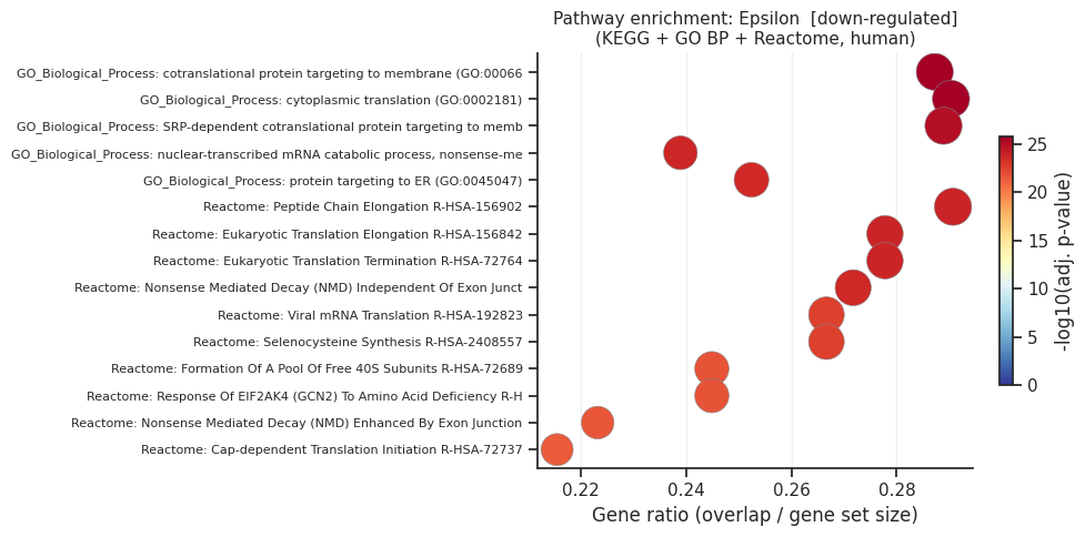
[down] Significant terms: 361
Gene_set Term Overlap Adjusted P-value
GO_Biological_Process_2021 cotranslational protein targeting to membrane (GO:0006613) 27/94 1.419635e-26
GO_Biological_Process_2021 cytoplasmic translation (GO:0002181) 27/93 1.419635e-26
GO_Biological_Process_2021 SRP-dependent cotranslational protein targeting to membrane (GO:0006614) 26/90 9.147683e-26
Reactome_2022 Peptide Chain Elongation R-HSA-156902 25/86 1.231498e-24
Reactome_2022 Eukaryotic Translation Elongation R-HSA-156842 25/90 1.482618e-24
Reactome_2022 Eukaryotic Translation Termination R-HSA-72764 25/90 1.482618e-24
GO_Biological_Process_2021 nuclear-transcribed mRNA catabolic process, nonsense-mediated decay (GO:0000184) 27/113 1.781313e-24
Reactome_2022 Nonsense Mediated Decay (NMD) Independent Of Exon Junction Complex (EJC) R-HSA-975956 25/92 2.059459e-24
GO_Biological_Process_2021 protein targeting to ER (GO:0045047) 26/103 2.772652e-24
Reactome_2022 Viral mRNA Translation R-HSA-192823 24/90 2.428940e-23
| fate | direction | Gene_set | Term | Overlap | Adjusted P-value | |
|---|---|---|---|---|---|---|
| 0 | Alpha | up | KEGG_2019_Mouse | Protein processing in endoplasmic reticulum | 17/163 | 3.014548e-06 |
| 1 | Alpha | up | KEGG_2019_Mouse | Thyroid hormone synthesis | 10/73 | 1.267707e-04 |
| 2 | Alpha | up | KEGG_2019_Mouse | Lysosome | 12/124 | 3.133244e-04 |
| 3 | Alpha | down | GO_Biological_Process_2021 | cotranslational protein targeting to membrane ... | 24/94 | 1.627570e-17 |
| 4 | Alpha | down | GO_Biological_Process_2021 | cytoplasmic translation (GO:0002181) | 24/93 | 1.627570e-17 |
| ... | ... | ... | ... | ... | ... | ... |
| 16 | Epsilon | up | Reactome_2022 | Peptide Hormone Metabolism R-HSA-2980736 | 10/89 | 1.607304e-04 |
| 17 | Epsilon | up | Reactome_2022 | Aberrant Regulation Of Mitotic G1/S Transition... | 5/17 | 4.275598e-04 |
| 18 | Epsilon | down | GO_Biological_Process_2021 | cotranslational protein targeting to membrane ... | 27/94 | 1.419635e-26 |
| 19 | Epsilon | down | GO_Biological_Process_2021 | cytoplasmic translation (GO:0002181) | 27/93 | 1.419635e-26 |
| 20 | Epsilon | down | GO_Biological_Process_2021 | SRP-dependent cotranslational protein targetin... | 26/90 | 9.147683e-26 |
21 rows × 6 columns
[32]:
# ── Custom gene sets ──────────────────────────────────────────────────────
# You can specify any Enrichr library:
# https://maayanlab.cloud/Enrichr/#libraries

custom_gene_sets = [
    'KEGG_2019_Mouse',
    'GO_Biological_Process_2021',
    'GO_Molecular_Function_2021',
    'Reactome_2022',
    'WikiPathway_2021_Mouse',
]

# enrichment = scorer.get_enrichment(
#     deg_drivers,
#     gene_sets=custom_gene_sets,
#     organism='mouse',
# )
print("Custom gene sets configured (commented out to avoid API call with synthetic data).")
print(f"Available sets: {custom_gene_sets}")
Custom gene sets configured (commented out to avoid API call with synthetic data).
Available sets: ['KEGG_2019_Mouse', 'GO_Biological_Process_2021', 'GO_Molecular_Function_2021', 'Reactome_2022', 'WikiPathway_2021_Mouse']
[33]:
# Export enrichment tables to CSV
try:
    scCS.export_enrichment_tables(enrichment, output_dir="enrichment_results/")
    print("Tables saved to enrichment_results/")
except Exception as e:
    print(f"Export skipped: {e}")
Saved: enrichment_results/enrichment_Alpha_up.csv
Saved: enrichment_results/enrichment_Alpha_down.csv
Saved: enrichment_results/enrichment_Beta_up.csv
Saved: enrichment_results/enrichment_Beta_down.csv
Saved: enrichment_results/enrichment_Delta_up.csv
Saved: enrichment_results/enrichment_Epsilon_up.csv
Saved: enrichment_results/enrichment_Epsilon_down.csv
Tables saved to enrichment_results/
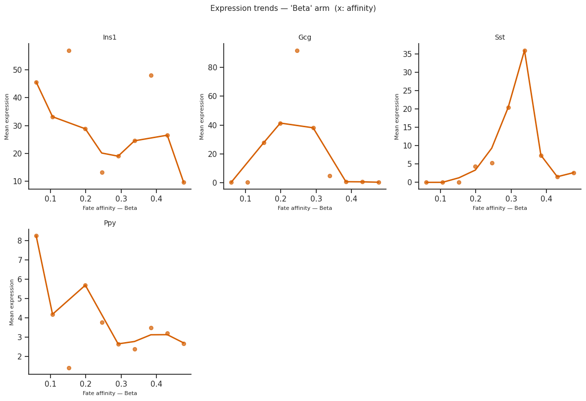
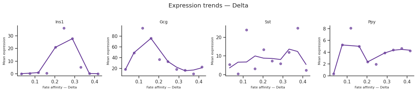
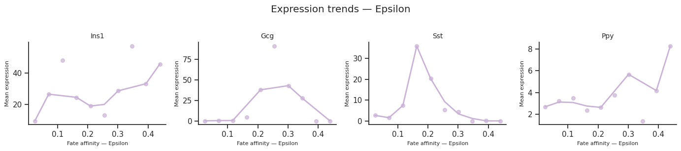
13. Expression trends along fate arms
plot_expression_trends() shows how gene expression changes along each fate arm, ordered by a differentiation metric.
The x_axis parameter controls the ordering:
'affinity'(default) — per-cell fate affinity score'pseudotime'— subset-local pseudotime'radial_distance'— distance from origin in the star embedding
[34]:
# Pick a few marker genes
genes_of_interest = ["Ins1", "Gcg", "Sst", "Ppy"]  # Beta, Alpha, Delta, Epsilon markers

# Expression trends ordered by fate affinity
# Signature: plot_expression_trends(adata_sub, result, genes, x_axis=...)
try:
    fig = scCS.plot_expression_trends(
        scorer.adata_sub,
        result,
        genes=genes_of_interest,
        x_axis="affinity",   # or 'pseudotime' or 'radial_distance'
        figsize=(12, 8),
    )
    plt.tight_layout()
    plt.show()
except Exception as e:
    print(f"Expression trends skipped: {e}")
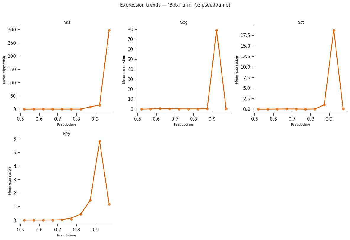
[35]:
# Ordered by pseudotime
try:
    fig = scCS.plot_expression_trends(
        scorer.adata_sub,
        result,
        genes=genes_of_interest,
        x_axis="pseudotime",
        figsize=(12, 8),
    )
    plt.tight_layout()
    plt.show()
except Exception as e:
    print(f"Expression trends skipped: {e}")
[36]:
obs_key = "clusters"   # <-- change to your obs column

color_map = dict(zip(
    adata.obs[obs_key].cat.categories,
    adata.uns[f"{obs_key}_colors"],
))
print(color_map)
{'Ductal': '#8fbc8f', 'Ngn3 low EP': '#f4a460', 'Ngn3 high EP': '#fdbf6f', 'Pre-endocrine': '#ff7f00', 'Beta': '#b2df8a', 'Alpha': '#1f78b4', 'Delta': '#6a3d9a', 'Epsilon': '#cab2d6'}
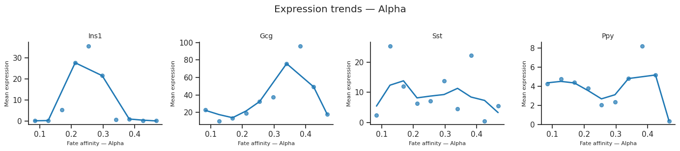
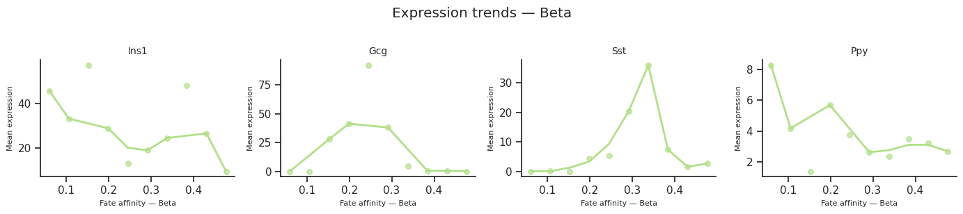
[37]:
for fate_name in result.fate_names:
    fig = scCS.plot_expression_trends(
        adata, result,
        genes=genes_of_interest,
        fate=fate_name,
        color_map=color_map,
        ncols=4,
    )
    fig.suptitle(f"Expression trends — {fate_name}", y=1.02)
    fig.savefig(f"expression_trends_{fate_name}.svg", bbox_inches="tight")
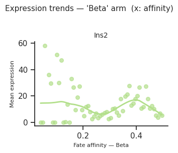
[38]:
# CellRank-style: cells binned by per-cell CS for a chosen fate,
# mean expression per bin plotted with LOWESS smooth.
# Requires compute_cell_level=True (Cell 2 above).

genes_of_interest = ["Ins2"]   # <-- your genes

fig = scCS.plot_expression_trends(
    adata,
    result,
    genes=genes_of_interest,
    fate=result.dominant_fate,   # or e.g. fate="Activated"
    n_bins=60,                   # bins along CS axis
    layer=None,             # or None to use adata.X
    smooth=True,
    smooth_frac=0.4,             # LOWESS bandwidth (0–1)
    color_map=color_map,
    ncols=2,
)
plt.show()
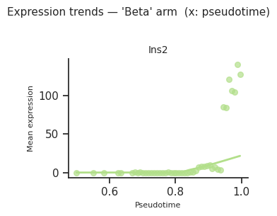
[39]:
fig = scCS.plot_expression_trends(
    adata,
    result,
    genes=genes_of_interest,
    fate=result.dominant_fate,   # or e.g. fate="Activated"
    n_bins=60,                   # bins along CS axis
    layer=None,             # or None to use adata.X
    smooth=True,
    smooth_frac=0.4,             # LOWESS bandwidth (0–1)
    color_map=color_map,
    ncols=2, x_axis="pseudotime",
)
plt.show()
Summary — scCS single-condition workflow
import scCS

# 1. Create scorer
scorer = scCS.SingleScorer(
    adata,
    root="Ductal",
    branches=["Alpha", "Beta", "Delta", "Epsilon"],
    obs_key="clusters",
)

# 2. Build embedding (fix arm coverage)
scorer.build_embedding(ordering_metric="pseudotime")
scorer.refit_pseudotime(scale_01=True)

# 3. Fit & score
scorer.fit()
result = scorer.score(cell_level=True, k_nn=15, n_bootstrap=500)
print(result.summary())

# 4. Visualize
scorer.plot_star(result)
scorer.plot_rose(result)
scorer.plot_pairwise_cs(result)
scorer.plot_commitment_bar(result)

# 5. Transfer labels to full adata
scorer.transfer_labels(adata, result)

# 6. Driver genes & enrichment
vel_drivers = scorer.get_velocity_drivers()
deg_drivers = scorer.get_deg_drivers()
enrichment  = scorer.get_enrichment(deg_drivers, organism="Human")
For multi-condition analysis, see the companion notebooks