scCS Tutorial — Pairwise Condition Comparison¶
Multi-Condition Commitment Score Analysis with PairScorer¶
This notebook demonstrates the multi-condition analysis workflow in scCS v0.7.0.
We artificially split the pancreas dataset into two groups:
“high_velocity” — cells with above-median RNA velocity magnitude (stronger commitment signal)
“low_velocity” — cells with below-median RNA velocity magnitude (weaker commitment signal)
This simulates a treatment effect where one condition drives stronger fate commitment.
Three-tier analysis framework¶
Tier |
What it answers |
Key functions |
|---|---|---|
Tier 1 |
What are the commitment scores per condition? |
|
Tier 2 |
Is the difference statistically significant? |
|
Tier 3 |
Does the trajectory shift between conditions? |
|
Reference¶
Kriukov et al. (2025) Single-cell transcriptome of myeloid cells in response to transplantation of human retinal neurons reveals reversibility of microglial activation
1. Setup and data loading¶
[1]:
%matplotlib inline
import numpy as np
import pandas as pd
import matplotlib.pyplot as plt
import scanpy as sc
import scvelo as scv

import warnings
warnings.filterwarnings("ignore", category=DeprecationWarning)
warnings.filterwarnings("ignore", category=FutureWarning)
try:
    from statsmodels.tools.sm_exceptions import ConvergenceWarning
    warnings.filterwarnings("ignore", category=ConvergenceWarning)
except ImportError:
    pass

import scCS

print(f"scCS version: {scCS.__version__}")

sc.settings.verbosity = 1
scv.settings.verbosity = 1

# --- Tutorial display helpers (compact tables instead of per-fate loops) ---
pd.set_option("display.max_rows", 25)
pd.set_option("display.max_columns", 15)
pd.set_option("display.width", 160)


def _stack_drivers_by_condition(driver_dicts, n_per_fate=5, cols=None):
    """Stack {condition: {fate: DataFrame}} into one tidy long-form table.

    Adds ``condition`` and ``fate`` columns at the front; shows top
    ``n_per_fate`` rows per (condition, fate) group.
    """
    out = []
    for cond, fate_dict in driver_dicts.items():
        for fate, df in fate_dict.items():
            if df is None or len(df) == 0:
                continue
            block = df.head(n_per_fate).copy()
            block.insert(0, "fate", fate)
            block.insert(0, "condition", cond)
            out.append(block)
    if not out:
        return pd.DataFrame()
    big = pd.concat(out, ignore_index=True)
    if cols is not None:
        keep = ["condition", "fate"] + [c for c in cols if c in big.columns]
        big = big[keep]
    return big


def _stack_enrichment_by_condition(enrichment_dicts, n_per_group=3):
    """Flatten {condition: {fate: {direction: df}}} into one tidy table."""
    rows = []
    for cond, fate_results in enrichment_dicts.items():
        for fate, dir_results in fate_results.items():
            for direction in ("up", "down"):
                df = dir_results.get(direction, None)
                if df is None or df.empty:
                    continue
                top = df.head(n_per_group).copy()
                top.insert(0, "direction", direction)
                top.insert(0, "fate", fate)
                top.insert(0, "condition", cond)
                rows.append(top)
    if not rows:
        return pd.DataFrame()
    return pd.concat(rows, ignore_index=True)


def _driver_overlap(per_cond_drivers, n_top=10, gene_col="gene"):
    """Build a fate x gene x condition presence matrix from {cond: {fate: df}}."""
    rows = []
    conds = list(per_cond_drivers.keys())
    if not conds:
        return pd.DataFrame()
    fates = list(next(iter(per_cond_drivers.values())).keys())
    for fate in fates:
        sets = {}
        for cond in conds:
            df = per_cond_drivers[cond].get(fate)
            if df is None or len(df) == 0 or gene_col not in df.columns:
                sets[cond] = set()
            else:
                sets[cond] = set(df.head(n_top)[gene_col].astype(str))
        all_genes = sorted(set.union(*sets.values())) if sets else []
        for g in all_genes:
            row = {"fate": fate, "gene": g}
            for cond in conds:
                row[cond] = g in sets[cond]
            row["n_conds"] = sum(row[c] for c in conds)
            row["shared_all"] = row["n_conds"] == len(conds)
            rows.append(row)
    return pd.DataFrame(rows)
scCS version: 0.7.4
[2]:
# Load the pancreas dataset
adata = scv.datasets.pancreas()

# Standard preprocessing
import inspect as _inspect
_fn_sig = _inspect.signature(scv.pp.filter_and_normalize).parameters
if "n_top_genes" in _fn_sig:
    scv.pp.filter_and_normalize(adata, min_shared_counts=20, n_top_genes=2000)
else:
    # scvelo builds without n_top_genes: do filter_and_normalize then HVG.
    # Use flavor="cell_ranger" not the default "seurat": seurat passes
    # int n_bins to pd.cut on log-dispersions which contain +/-inf for
    # low-mean genes — pandas >= 2.2 rejects this with ValueError.
    # cell_ranger uses explicit bin edges including +/-inf and is
    # robust across pandas/py versions (scCS changelog v0.7.4).
    scv.pp.filter_and_normalize(adata, min_shared_counts=20)
    sc.pp.highly_variable_genes(
        adata, n_top_genes=2000, subset=True, flavor="cell_ranger"
    )
sc.pp.neighbors(adata)
scv.pp.moments(adata, n_pcs=None, n_neighbors=None)

print(adata)
AnnData object with n_obs × n_vars = 3696 × 2000
    obs: 'clusters_coarse', 'clusters', 'S_score', 'G2M_score', 'initial_size_unspliced', 'initial_size_spliced', 'initial_size', 'n_counts'
    var: 'highly_variable_genes', 'gene_count_corr', 'highly_variable', 'means', 'dispersions', 'dispersions_norm'
    uns: 'clusters_coarse_colors', 'clusters_colors', 'day_colors', 'neighbors', 'pca', 'hvg'
    obsm: 'X_pca', 'X_umap'
    layers: 'spliced', 'unspliced', 'Ms', 'Mu'
    obsp: 'distances', 'connectivities'
[3]:
# Run RNA velocity (dynamical model)
scv.tl.recover_dynamics(adata, n_jobs=32)
scv.tl.velocity(adata, mode="dynamical")
scv.tl.velocity_graph(adata)
scv.tl.velocity_pseudotime(adata)

print("Velocity computed.")
/home/emil/miniforge3/envs/lab-py312/lib/python3.12/multiprocessing/popen_fork.py:66: DeprecationWarning: This process (pid=4708) is multi-threaded, use of fork() may lead to deadlocks in the child.
  self.pid = os.fork()
/home/emil/miniforge3/envs/lab-py312/lib/python3.12/multiprocessing/popen_fork.py:66: DeprecationWarning: This process (pid=4708) is multi-threaded, use of fork() may lead to deadlocks in the child.
  self.pid = os.fork()
Velocity computed.
2. Create artificial condition split¶
We split cells into two groups based on their RNA velocity magnitude:
high_velocity — cells with above-median velocity magnitude
low_velocity — cells with below-median velocity magnitude
This simulates a scenario where a treatment (e.g., a drug or genetic perturbation) increases the strength of fate commitment signals.
In a real experiment,
condition_obs_keywould point to a column like'treatment','genotype', or'time_point'already present inadata.obs.
[4]:
# Compute per-cell velocity magnitude from the velocity layer
velocity_matrix = adata.layers["velocity"]  # shape: (n_cells, n_genes)
# Use RMS across genes as a per-cell magnitude proxy
vel_magnitude = np.sqrt(np.nanmean(velocity_matrix ** 2, axis=1))

# Split at the median
median_mag = np.median(vel_magnitude)
adata.obs["condition"] = np.where(
    vel_magnitude >= median_mag, "high_velocity", "low_velocity"
)

# Also create a fake replicate column (for mixed model demo)
# In practice this would be biological replicates / samples
np.random.seed(42)
adata.obs["sample"] = np.random.choice(
    ["rep1", "rep2", "rep3"], size=adata.n_obs
)

print("Condition distribution:")
print(adata.obs["condition"].value_counts())
print("\nSample distribution:")
print(adata.obs["sample"].value_counts())
Condition distribution:
condition
high_velocity    1848
low_velocity     1848
Name: count, dtype: int64

Sample distribution:
sample
rep1    1282
rep2    1224
rep3    1190
Name: count, dtype: int64
[5]:
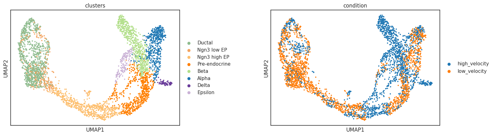
# Visualize the split on UMAP
sc.pl.umap(adata, color=["condition", "clusters"], ncols=2, wspace=0.4,
           title=["Artificial condition split", "Cell clusters"])
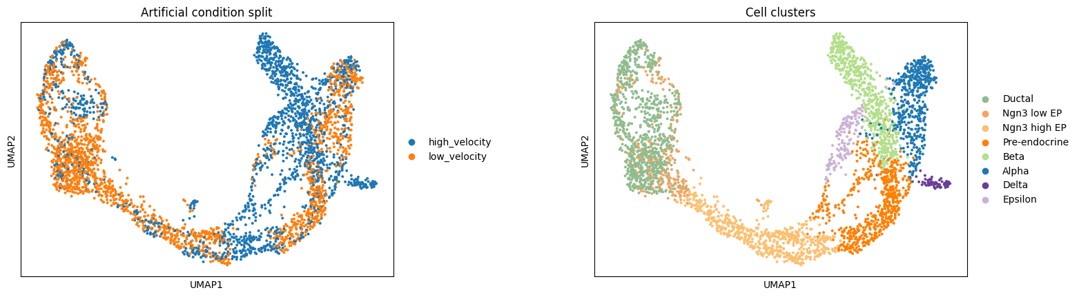
[6]:
# Confirm both conditions contain bifurcation + terminal fate cells
for cond in ["high_velocity", "low_velocity"]:
    sub = adata[adata.obs["condition"] == cond]
    clusters_present = sub.obs["clusters"].unique().tolist()
    print(f"\n{cond}: {sub.n_obs} cells")
    print(f"  Clusters: {sorted(clusters_present)}")
high_velocity: 1848 cells
  Clusters: ['Alpha', 'Beta', 'Delta', 'Ductal', 'Epsilon', 'Ngn3 high EP', 'Ngn3 low EP', 'Pre-endocrine']

low_velocity: 1848 cells
  Clusters: ['Alpha', 'Beta', 'Ductal', 'Epsilon', 'Ngn3 high EP', 'Ngn3 low EP', 'Pre-endocrine']
3. Initialize PairScorer¶
PairScorer wraps SingleScorer and builds a shared embedding on pooled data from all conditions. This ensures that arm geometry is identical across conditions — a prerequisite for valid cross-condition comparison.
Key parameters:
condition_obs_key— column inadata.obswith condition labelsAll other parameters are identical to
SingleScorer
[7]:
mscorer = scCS.PairScorer(
    adata,
    root="Pre-endocrine",
    branches=["Alpha", "Beta", "Delta", "Epsilon"],
    condition_obs_key="condition",   # our artificial split
    obs_key="clusters",
    n_angle_bins=36,
    sector_method="centroid",
)
[scCS] PairScorer initialized.
       Conditions (2): ['high_velocity', 'low_velocity']
       Root: 'Pre-endocrine', Branches: ['Alpha', 'Beta', 'Delta', 'Epsilon']
Tier 1: Score each condition on the shared embedding¶
score_all_conditions() computes commitment scores separately for each condition, using the shared embedding and FateMap. Each condition’s cells are masked from the shared adata_sub.
[10]:
# Score all conditions
results = mscorer.score_all_conditions(
    cell_level=True,
    k_nn=15,
    n_bootstrap=200,   # bootstrap CI per condition
    bootstrap_ci=0.95,
    verbose=True,
)
[scCS] Scoring condition: 'high_velocity' (1249 cells)...
[scCS] Computing bootstrap CI (n=200)...
=== CommitmentScoreResult ===
  Fates (4): Alpha, Beta, Delta, Epsilon
  Dominant fate: Beta

  Entropy metrics:
    Population entropy:           0.6209  [aggregate velocity-mass balance]
    Mean cell entropy:            0.9361  [per-cell average, k-way]
    Per-fate cell entropy:
      Alpha: 0.8246
      Beta: 0.8608
      Delta: 0.7541
      Epsilon: 0.6399
    NN-smoothed entropy (k=15):  mean=0.9547  [per-cell, stored in adata_sub.obs['cs_nn_entropy']]

  Commitment vector (normalized):
    Alpha: 0.1490
    Beta: 0.7267
    Delta: 0.0663
    Epsilon: 0.0580

  Pairwise nCS matrix:
            Alpha      Beta     Delta   Epsilon
Alpha    1.000000  0.539098  0.756585  1.443795
Beta     1.854951  1.000000  1.403429  2.678169
Delta    1.321728  0.712540  1.000000  1.908304
Epsilon  0.692619  0.373389  0.524026  1.000000

  Bootstrap 95% CI on nCS (n=200):
    CI low:
         Alpha   Beta  Delta  Epsilon
Alpha    1.000  0.462  0.589    1.118
Beta     1.616  1.000  1.175    2.170
Delta    1.021  0.581  1.000    1.422
Epsilon  0.528  0.293  0.401    1.000
    CI high:
         Alpha   Beta  Delta  Epsilon
Alpha    1.000  0.619  0.979    1.895
Beta     2.163  1.000  1.722    3.416
Delta    1.699  0.851  1.000    2.492
Epsilon  0.894  0.461  0.703    1.000

[scCS] Scoring condition: 'low_velocity' (627 cells)...
[scCS] Computing bootstrap CI (n=200)...
=== CommitmentScoreResult ===
  Fates (4): Alpha, Beta, Delta, Epsilon
  Dominant fate: Alpha

  Entropy metrics:
    Population entropy:           0.8152  [aggregate velocity-mass balance]
    Mean cell entropy:            0.9361  [per-cell average, k-way]
    Per-fate cell entropy:
      Alpha: 0.8246
      Beta: 0.8608
      Delta: 0.7541
      Epsilon: 0.6399
    NN-smoothed entropy (k=15):  mean=0.9547  [per-cell, stored in adata_sub.obs['cs_nn_entropy']]

  Commitment vector (normalized):
    Alpha: 0.4481
    Beta: 0.3870
    Delta: 0.1087
    Epsilon: 0.0562

  Pairwise nCS matrix:
            Alpha      Beta  Delta   Epsilon
Alpha    1.000000  0.186620    0.0  0.730455
Beta     5.358472  1.000000    0.0  3.914121
Delta         inf       inf    1.0       inf
Epsilon  1.369010  0.255485    0.0  1.000000
  (inf = fate arm has 0 cells in this subset; expected for progenitor-only subsets)

  Bootstrap 95% CI on nCS (n=200):
    CI low:
         Alpha   Beta  Delta  Epsilon
Alpha    1.000  0.150    0.0    0.530
Beta     4.189  1.000    0.0    2.757
Delta      NaN    NaN    1.0      NaN
Epsilon  0.916  0.168    0.0    1.000
    CI high:
         Alpha   Beta  Delta  Epsilon
Alpha    1.000  0.239    0.0    1.092
Beta     6.677  1.000    0.0    5.940
Delta      NaN    NaN    1.0      NaN
Epsilon  1.887  0.363    0.0    1.000
[11]:
# Compare nCS matrices side by side
for cond, res in results.items():
    print(f"\n=== {cond} ===")
    print(pd.DataFrame(
        res.pairwise_nCS,
        index=res.fate_names,
        columns=res.fate_names
    ).round(3))
=== high_velocity ===
         Alpha   Beta  Delta  Epsilon
Alpha    1.000  0.539  0.757    1.444
Beta     1.855  1.000  1.403    2.678
Delta    1.322  0.713  1.000    1.908
Epsilon  0.693  0.373  0.524    1.000

=== low_velocity ===
         Alpha   Beta  Delta  Epsilon
Alpha    1.000  0.187    0.0    0.730
Beta     5.358  1.000    0.0    3.914
Delta      inf    inf    1.0      inf
Epsilon  1.369  0.255    0.0    1.000
[12]:
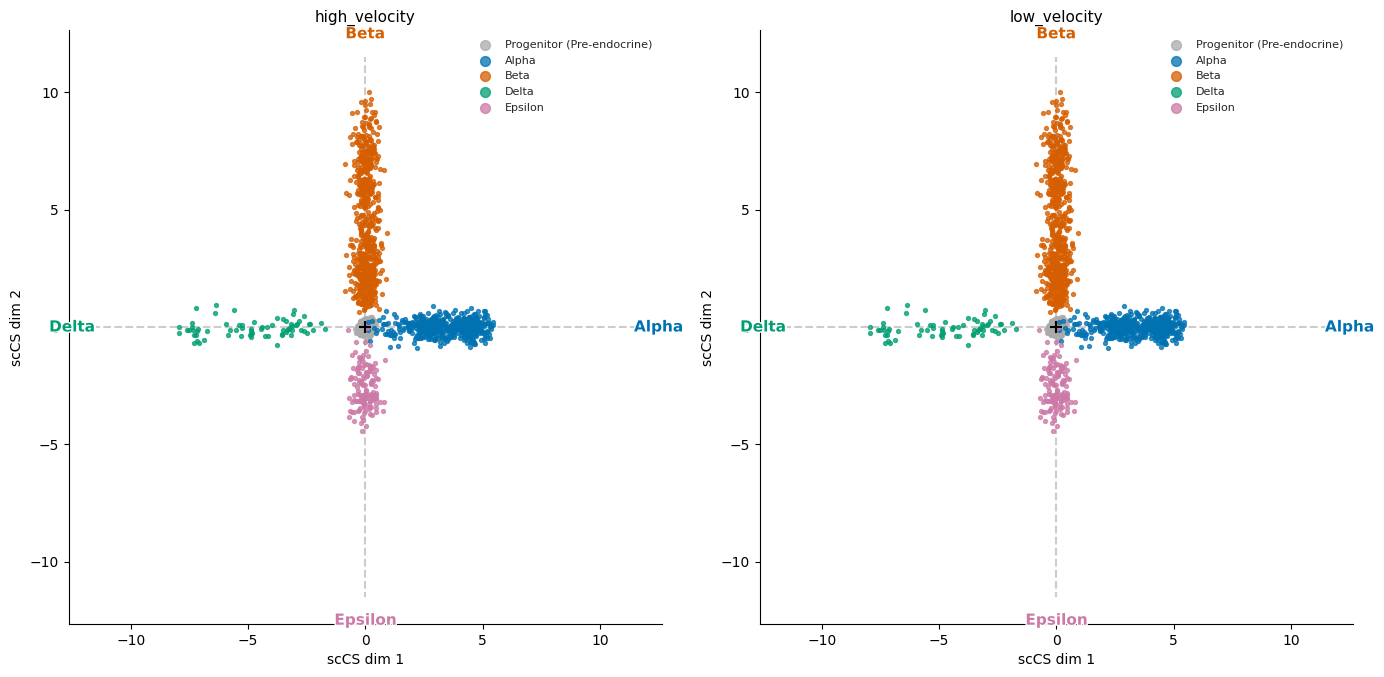
# Side-by-side star plots for each condition
# figsize_per_panel controls the size of each individual panel
fig = mscorer.plot_star_grid(
    results,
    figsize_per_panel=(7, 7),
)
plt.tight_layout()
plt.show()
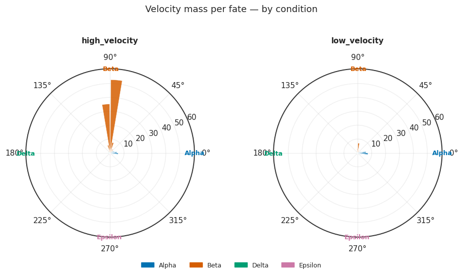
Tier 1b: Per-condition rose plots¶
plot_rose_grid() shows one polar rose plot per condition, all panels sharing the same radial scale for direct magnitude comparison across conditions.
[13]:
# Per-condition rose plots (shared radial scale)
fig = mscorer.plot_rose_grid(
    results,
    figsize_per_panel=(5, 5),
    title="Velocity mass per fate — by condition",
)
plt.tight_layout()
plt.show()
[14]:
# Commitment vectors per condition
print("Commitment vectors (fraction of velocity mass per fate):")
for cond, res in results.items():
    print(f"\n  {cond}:")
    for fate, cv in zip(res.fate_names, res.commitment_vector):
        print(f"    {fate}: {cv:.3f}")
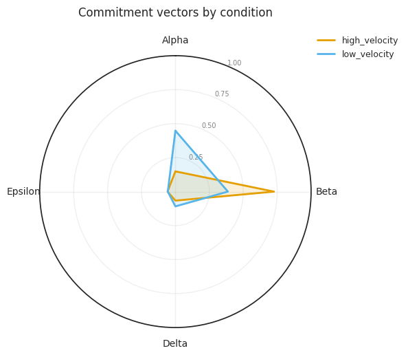
Commitment vectors (fraction of velocity mass per fate):

  high_velocity:
    Alpha: 0.149
    Beta: 0.727
    Delta: 0.066
    Epsilon: 0.058

  low_velocity:
    Alpha: 0.448
    Beta: 0.387
    Delta: 0.109
    Epsilon: 0.056
Tier 2: Statistical comparison¶
2a. ΔCS with bootstrap confidence intervals¶
compute_delta_CS() computes ΔnCS = nCS_A − nCS_B for each fate pair, with bootstrap CIs obtained by resampling cells within each condition.
A CI that does not include 0 indicates a statistically meaningful difference.
[15]:
# Compute ΔCS: high_velocity − low_velocity
delta = mscorer.compute_delta_CS(
    condition_a="high_velocity",
    condition_b="low_velocity",
    n_bootstrap=500,
    ci=0.95,
    verbose=True,
)
=== ΔCS: 'high_velocity' − 'low_velocity' ===
  ΔnCS (point estimate):
         Alpha   Beta  Delta  Epsilon
Alpha    0.000  0.352  0.757    0.713
Beta    -3.504  0.000  1.403   -1.236
Delta     -inf   -inf  0.000     -inf
Epsilon -0.676  0.118  0.524    0.000

  95% CI low:
         Alpha   Beta  Delta  Epsilon
Alpha    0.000  0.279  0.640    0.317
Beta    -4.659  0.000  1.210   -2.743
Delta      NaN    NaN  0.000      NaN
Epsilon -1.115  0.013  0.422    0.000

  95% CI high:
         Alpha   Beta  Delta  Epsilon
Alpha    0.000  0.425  0.921    1.070
Beta    -2.506  0.000  1.667   -0.106
Delta      NaN    NaN  0.000      NaN
Epsilon -0.259  0.209  0.654    0.000
[16]:
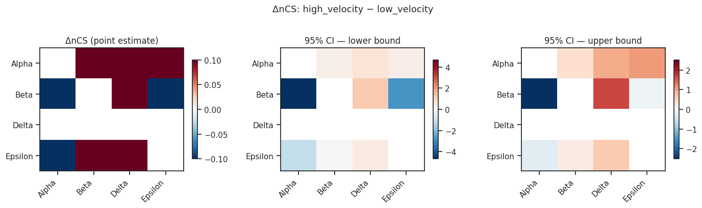
# Visualize ΔCS as a heatmap
import matplotlib.pyplot as plt
import matplotlib.colors as mcolors

fate_names = delta["fate_names"]
k = len(fate_names)
delta_mat = delta["delta_nCS"]
ci_low = delta["ci_low"]
ci_high = delta["ci_high"]

fig, axes = plt.subplots(1, 3, figsize=(14, 4))

for ax, mat, title in zip(
    axes,
    [delta_mat, ci_low, ci_high],
    ["ΔnCS (point estimate)", "95% CI — lower bound", "95% CI — upper bound"]
):
    # Mask diagonal
    masked = np.where(np.eye(k, dtype=bool), np.nan, mat)
    vmax = np.nanmax(np.abs(masked))
    im = ax.imshow(masked, cmap="RdBu_r", vmin=-vmax, vmax=vmax, aspect="auto")
    ax.set_xticks(range(k)); ax.set_xticklabels(fate_names, rotation=45, ha="right")
    ax.set_yticks(range(k)); ax.set_yticklabels(fate_names)
    ax.set_title(title)
    plt.colorbar(im, ax=ax, shrink=0.8)

plt.suptitle("ΔnCS: high_velocity − low_velocity", fontsize=13, y=1.02)
plt.tight_layout()
plt.show()
[17]:
# Identify fate pairs where CI excludes 0 (significant differences)
print("Fate pairs with significant ΔnCS (95% CI excludes 0):")
for i, fi in enumerate(fate_names):
    for j, fj in enumerate(fate_names):
        if i >= j:
            continue
        lo, hi = ci_low[i, j], ci_high[i, j]
        if lo > 0 or hi < 0:
            direction = "↑" if delta_mat[i, j] > 0 else "↓"
            print(f"  {fi} vs {fj}: Δ={delta_mat[i,j]:.3f} [{lo:.3f}, {hi:.3f}] {direction}")
Fate pairs with significant ΔnCS (95% CI excludes 0):
  Alpha vs Beta: Δ=0.352 [0.279, 0.425] ↑
  Alpha vs Delta: Δ=0.757 [0.640, 0.921] ↑
  Alpha vs Epsilon: Δ=0.713 [0.317, 1.070] ↑
  Beta vs Delta: Δ=1.403 [1.210, 1.667] ↑
  Beta vs Epsilon: Δ=-1.236 [-2.743, -0.106] ↓
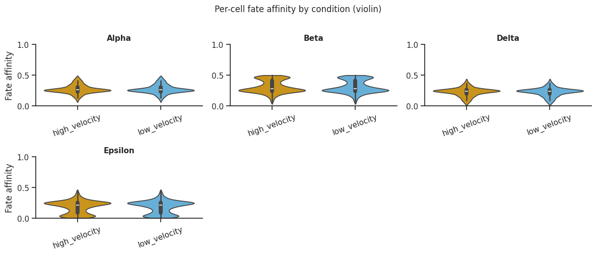
2b. Permutation test on per-cell fate affinities¶
compare_conditions() tests whether per-cell fate affinity scores differ significantly between conditions.
k=2 conditions: permutation test (shuffle condition labels, recompute mean difference)
k>2 conditions: Kruskal-Wallis + pairwise Mann-Whitney U with Bonferroni correction
[18]:
# Statistical comparison of per-cell fate affinities
stats_df = mscorer.compare_conditions(
    results,
    test="auto",          # 'permutation' for k=2, 'kruskal' for k>2
    n_permutations=1000,
    pval_threshold=0.05,
    verbose=True,
)

print("\nStatistical comparison results:")
print(stats_df.to_string(index=False))
=== Condition comparison ===
  Test: auto  |  Significant results: 0 / 4
  No significant differences at pval_adj < 0.05.

Statistical comparison results:
   fate                    comparison           test  statistic  pval   mean_A   mean_B  pval_adj  significant
  Alpha high_velocity vs low_velocity kruskal-wallis        0.0   1.0 0.270815 0.270815       1.0        False
   Beta high_velocity vs low_velocity kruskal-wallis        0.0   1.0 0.312566 0.312566       1.0        False
  Delta high_velocity vs low_velocity kruskal-wallis        0.0   1.0 0.228806 0.228806       1.0        False
Epsilon high_velocity vs low_velocity kruskal-wallis        0.0   1.0 0.187813 0.187813       1.0        False
[19]:
# Violin / box / strip plots of per-cell fate affinities
fig = mscorer.plot_affinity_distributions(
    results,
    plot_type="violin",   # 'violin', 'box', or 'strip'
    figsize=(12, 5),
)
plt.tight_layout()
plt.show()
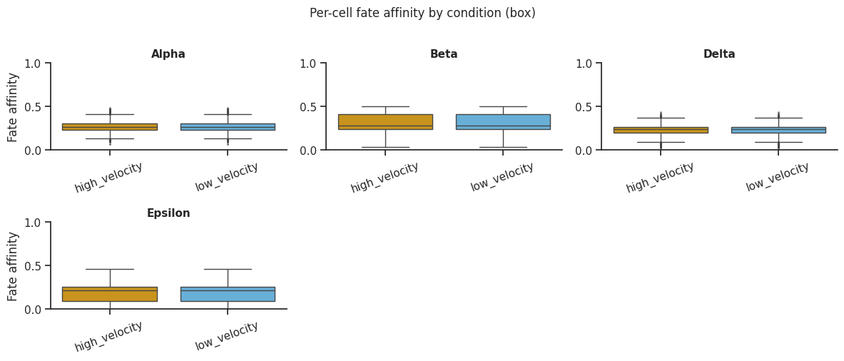
[20]:
# Box plot version
fig = mscorer.plot_affinity_distributions(
    results,
    plot_type="box",
    figsize=(12, 5),
)
plt.tight_layout()
plt.show()
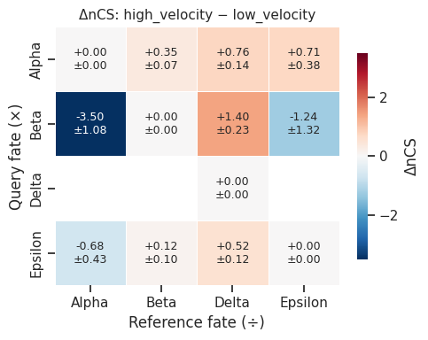
2c. Additional multi-condition visualizations¶
Three new plots for comparing commitment across conditions:
``plot_delta_cs_heatmap()`` — diverging heatmap of ΔnCS annotated with Δ ± CI
``plot_compare_conditions_bar()`` — grouped bar chart of nCS per condition per fate pair
``plot_commitment_vector_radar()`` — radar/spider chart of commitment vectors
[21]:
# ΔCS heatmap with CI annotation
fig = mscorer.plot_delta_cs_heatmap(
    delta,
    title="ΔnCS: high_velocity − low_velocity",
    figsize=(5, 4),
)
plt.tight_layout()
plt.show()
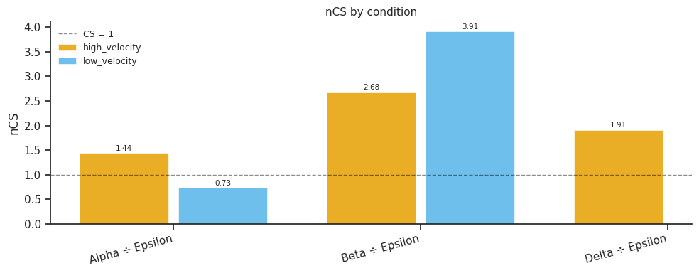
[22]:
# Grouped bar chart: nCS per condition per fate pair
fig = mscorer.plot_compare_conditions_bar(
    results,
    title="nCS by condition",
    figsize=(10, 4),
)
plt.tight_layout()
plt.show()
[23]:
# Radar chart of commitment vectors (one polygon per condition)
# Falls back to bar chart for k < 3
fig = mscorer.plot_commitment_vector_radar(
    results,
    title="Commitment vectors by condition",
    figsize=(6, 6),
)
plt.tight_layout()
plt.show()
Tier 3: Trajectory-level analysis¶
3a. Mixed linear model¶
fit_mixed_model() fits a linear mixed model (via statsmodels MixedLM) for each fate arm:
affinity ~ condition  (fixed effect)
         + (1 | sample)  (random effect — accounts for replicate variation)
This is the most rigorous approach when you have biological replicates.
[24]:
# Fit mixed model: condition fixed effect, sample random effect
try:
    lmm_results = mscorer.fit_mixed_model(
        results,
        replicate_key="sample",   # replicate column
        verbose=True,
    )

    print("\nMixed model results:")
    print(lmm_results.to_string(index=False))
except Exception as e:
    print(f"Mixed model skipped (requires statsmodels): {e}")
=== Mixed-effects model results ===
  Significant effects: 0 / 4

Mixed model results:
   fate    condition     reference          coef  std_err       z_score  pval    ci_low  ci_high  pval_adj  significant
  Alpha low_velocity high_velocity -3.254918e-19 0.002280 -1.427620e-16   1.0 -0.004469 0.004469       1.0        False
   Beta low_velocity high_velocity -1.775410e-18 0.003320 -5.346931e-16   1.0 -0.006508 0.006508       1.0        False
  Delta low_velocity high_velocity -1.220594e-18 0.002279 -5.354918e-16   1.0 -0.004468 0.004468       1.0        False
Epsilon low_velocity high_velocity  3.030033e-16 0.003302  9.177422e-14   1.0 -0.006471 0.006471       1.0        False
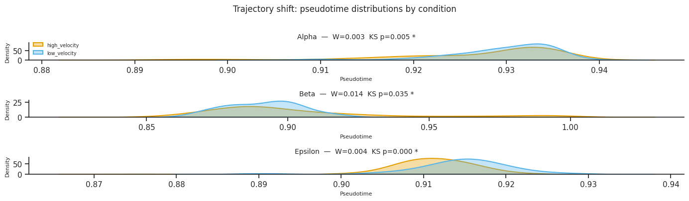
3b. Trajectory shift analysis¶
trajectory_shift() tests whether the pseudotime distribution along each fate arm differs between conditions using:
Kolmogorov-Smirnov (KS) test — detects any distributional difference
Wasserstein distance — quantifies the magnitude of the shift, with bootstrap CI
A significant KS test + large Wasserstein distance indicates that cells in one condition are systematically further along (or earlier in) the differentiation trajectory.
[25]:
# Trajectory shift analysis
# Returns a DataFrame with columns: fate, comparison, ks_stat, ks_pval,
# wasserstein, wasserstein_ci_low, wasserstein_ci_high, mean_pt_A, mean_pt_B,
# delta_mean_pt, significant
try:
    shift_df = mscorer.trajectory_shift(
        results,
        n_bootstrap=500,
        verbose=True,
    )

    print("\nTrajectory shift summary:")
    print(shift_df[["fate", "comparison", "ks_stat", "ks_pval",
                     "wasserstein", "wasserstein_ci_low", "wasserstein_ci_high",
                     "significant"]].to_string(index=False))
except Exception as e:
    print(f"Trajectory shift skipped: {e}")
    shift_df = None
=== Trajectory shift analysis ===
  Significant shifts: 3 / 3
   fate                    comparison  ks_stat  ks_pval_adj  wasserstein  delta_mean_pt
  Alpha high_velocity vs low_velocity 0.171245     0.005030     0.002727      -0.002664
   Beta high_velocity vs low_velocity 0.246261     0.034612     0.014225       0.012765
Epsilon high_velocity vs low_velocity 0.481026     0.000210     0.003927      -0.003627

Trajectory shift summary:
   fate                    comparison  ks_stat  ks_pval  wasserstein  wasserstein_ci_low  wasserstein_ci_high  significant
  Alpha high_velocity vs low_velocity 0.171245 0.001677     0.002727            0.001802             0.004006         True
   Beta high_velocity vs low_velocity 0.246261 0.011537     0.014225            0.012215             0.018473         True
Epsilon high_velocity vs low_velocity 0.481026 0.000070     0.003927            0.002510             0.006638         True
[26]:
# KDE plots of pseudotime distributions per fate per condition
try:
    if shift_df is not None:
        fig = mscorer.plot_trajectory_shift(
            shift_df,
            figsize=(14, 4),
        )
        plt.tight_layout()
        plt.show()
except Exception as e:
    print(f"Trajectory shift plot skipped: {e}")
6. Driver genes per condition¶
Identify fate-driving genes (velocity-based, DEG-based, velocity-fate correlation) within each condition. Use the shared adata_sub per condition, then assemble the results into one tidy table with (condition, fate) columns.
This is the standard way to find genes whose role in commitment changes between conditions: a gene that is a top driver in low_velocity but not in high_velocity is a candidate condition-specific regulator.
[27]:
# Velocity-based drivers — run per condition
from scCS.drivers import get_velocity_drivers

adata_sub_shared = mscorer._scorer.adata_sub
fate_names = mscorer._scorer._fate_map.fate_names
root_cluster = mscorer._scorer.root
obs_key_used = mscorer._scorer.obs_key

vel_drivers_per_cond = {}
for cond in mscorer.conditions:
    mask = (adata_sub_shared.obs[mscorer.condition_obs_key].astype(str) == cond).values
    sub = adata_sub_shared[mask].copy()
    vel_drivers_per_cond[cond] = get_velocity_drivers(
        sub, fate_names=fate_names, obs_key=obs_key_used,
        root=root_cluster, n_top_genes=20,
    )

# Compact long-form table
print("Top velocity drivers (top 5 per fate, per condition):")
_stack_drivers_by_condition(
    vel_drivers_per_cond, n_per_fate=5,
    cols=["gene", "mean_velocity", "rank"],
)
── Velocity drivers: Alpha (top 20, sorted by delta_velocity) ──
 rank    gene  delta_velocity  mean_velocity
    1     Clu        2.394982       2.601254
    2    Ghrl        2.230801       1.208408
    3  Btbd17        1.361021       1.130396
    4  Cryba2        1.165649       1.429237
    5    Cpa2        0.996341       0.808371
    6  Tm4sf4        0.752253       0.572645
    7  Npepl1        0.701914       0.203834
    8     Hn1        0.642953       0.173084
    9    Pax6        0.628259       0.938433
   10   Meis2        0.613610       0.691767
   11    Vasp        0.563599       0.066359
   12 Lurap1l        0.551248       0.355268
   13   Rgs17        0.542472       0.575468
   14   Celf3        0.540257       0.375474
   15    Tox3        0.529739       0.308918
   16   Cd200        0.518199       0.406608
   17  Ppp3ca        0.514993       0.219860
   18    Pax4        0.478970       0.058572
   19    Cpt2        0.421590       0.253768
   20 Smarcd2        0.420897       0.419561

── Velocity drivers: Beta (top 20, sorted by delta_velocity) ──
 rank          gene  delta_velocity  mean_velocity
    1          Isl1        4.461863       1.070405
    2          Ins2        3.953642       3.972451
    3          Nnat        3.673498       4.141401
    4           Clu        1.607484       1.813756
    5 1700086L19Rik        1.450399       0.549565
    6          Krt7        0.955820       0.266415
    7       Igfbpl1        0.847445       0.290844
    8        Tm4sf4        0.816697       0.637089
    9          Pax4        0.810044       0.389647
   10       Ppp1r1a        0.809831       1.533254
   11          Ghrl        0.779220      -0.243173
   12          Dbn1        0.643636       0.332081
   13       Smarcd2        0.605017       0.603681
   14          Pax6        0.562075       0.872248
   15          Cpa2        0.534046       0.346076
   16         Cldn6        0.472029      -0.293498
   17         Glud1        0.468660       0.732603
   18       Lurap1l        0.468362       0.272382
   19         Ccnd2        0.465604       0.394593
   20      BC023829        0.456752       0.379688

── Velocity drivers: Delta (top 20, sorted by delta_velocity) ──
 rank     gene  delta_velocity  mean_velocity
    1     Krt8        2.332098       1.407045
    2     Cpa2        2.280671       2.092702
    3   Maged2        1.876646       3.380898
    4     Ldha        1.703658       1.581080
    5   Cryba2        1.640011       1.903599
    6      Hn1        1.156748       0.686879
    7   Cdkn1c        1.062967       1.007896
    8     Nnat        1.012159       1.480061
    9     Ambp        0.976446       0.752210
   10  Ppp1r1a        0.971532       1.694955
   11     Gnas        0.935484       6.604826
   12    Rpl12        0.699341      -0.154604
   13     Pax6        0.698164       1.008338
   14    Sparc        0.694246       0.649847
   15    Krt18        0.678155      -0.206350
   16    Cotl1        0.649170       0.579984
   17    Celf3        0.638144       0.473361
   18 BC023829        0.593681       0.516617
   19  Akr1c19        0.585637       1.123999
   20    Foxa3        0.581431       0.411777

── Velocity drivers: Epsilon (top 20, sorted by delta_velocity) ──
 rank     gene  delta_velocity  mean_velocity
    1     Cpa2        1.433100       1.245131
    2   Cryba2        1.283010       1.546598
    3      Clu        1.193620       1.399892
    4    Meis2        0.974752       1.052909
    5    Siva1        0.751692       0.628769
    6   Btbd17        0.723855       0.493231
    7  Lurap1l        0.644486       0.448505
    8     Pax4        0.639611       0.219213
    9    Syt13        0.626162       0.824190
   10   Cdkn1c        0.600463       0.545391
   11     Pax6        0.599071       0.909244
   12    Rgs17        0.554066       0.587061
   13   Nudt19        0.540254       0.460169
   14  Arl6ip1        0.493820      -0.131398
   15     Cpt2        0.455947       0.288125
   16   Npepl1        0.448234      -0.049846
   17    Birc5        0.410141       0.374991
   18     Cdk1        0.397182       0.417446
   19      Tkt        0.378253       0.332503
   20 Ppp1r14b        0.371528      -0.291778

── Velocity drivers: Alpha (top 20, sorted by delta_velocity) ──
 rank     gene  delta_velocity  mean_velocity
    1     Cpa2        1.493780       0.883649
    2    Meis2        1.053937       0.645838
    3   Cryba2        1.008127       1.055581
    4     Pax6        0.848950       0.841338
    5      Clu        0.848731       0.717436
    6   Npepl1        0.757560       0.166575
    7     Pax4        0.744543       0.016807
    8     Krt7        0.716767      -0.259284
    9     Vasp        0.652932       0.121307
   10     Pdx1        0.634857       0.383033
   11   Tm4sf4        0.611374       0.384856
   12    Cd200        0.577635       0.271759
   13    Celf3        0.529539       0.366640
   14 BC023829        0.514373       0.350243
   15     Tox3        0.480100       0.207980
   16   Ppp3ca        0.463614       0.186181
   17    Map1b        0.459361       0.640919
   18     Krt8        0.457733      -0.503180
   19    Psmc2        0.454385      -0.456419
   20     Cpt2        0.447037       0.240750

── Velocity drivers: Beta (top 20, sorted by delta_velocity) ──
 rank     gene  delta_velocity  mean_velocity
    1     Isl1        2.591787       1.067878
    2     Nnat        2.565379       2.934238
    3     Krt7        1.673100       0.697048
    4    Meis2        1.406825       0.998726
    5     Hadh        1.254540       1.095723
    6  Ppp1r1a        0.992641       1.621375
    7   Tm4sf4        0.900606       0.674089
    8 BC023829        0.751555       0.587425
    9     Pax6        0.649637       0.642025
   10     Cpa2        0.648636       0.038504
   11    Spc24        0.624380       0.625219
   12  Lurap1l        0.589024       0.443184
   13    Glud1        0.556597       0.805027
   14  S100a10        0.545249       0.614486
   15     Dlk1        0.522090       1.872635
   16    Phgdh        0.512333       0.456298
   17    Syt13        0.506459       0.347345
   18    Map1b        0.486952       0.668510
   19    Peg10        0.480236       0.988289
   20     Gars        0.461482       0.495746

── Velocity drivers: Epsilon (top 20, sorted by delta_velocity) ──
 rank    gene  delta_velocity  mean_velocity
    1    Isl1        1.954779       0.430871
    2   Meis2        1.466027       1.057928
    3    Pax4        1.266948       0.539212
    4     Clu        1.176291       1.044996
    5  Cryba2        1.061596       1.109050
    6 Arl6ip1        1.010438       0.328101
    7   Syt13        0.989686       0.830572
    8    Pdx1        0.905458       0.653633
    9    Pax6        0.798171       0.790560
   10 Lurap1l        0.786681       0.640841
   11    Ghrl        0.706006       0.556429
   12 Runx1t1        0.666353       0.454053
   13   Siva1        0.663069       0.555349
   14   Cldn7        0.652394      -0.025911
   15     Tkt        0.628411       0.701861
   16  Nudt19        0.597660       0.495606
   17  Npepl1        0.578077      -0.012909
   18    Gars        0.554945       0.589210
   19 Akr1c19        0.540149       0.622992
   20    Nrep        0.521967       0.357101
Top velocity drivers (top 5 per fate, per condition):
[27]:
| condition | fate | gene | mean_velocity | rank | |
|---|---|---|---|---|---|
| 0 | high_velocity | Alpha | Clu | 2.601254 | 1 |
| 1 | high_velocity | Alpha | Ghrl | 1.208408 | 2 |
| 2 | high_velocity | Alpha | Btbd17 | 1.130396 | 3 |
| 3 | high_velocity | Alpha | Cryba2 | 1.429237 | 4 |
| 4 | high_velocity | Alpha | Cpa2 | 0.808371 | 5 |
| ... | ... | ... | ... | ... | ... |
| 30 | low_velocity | Epsilon | Isl1 | 0.430871 | 1 |
| 31 | low_velocity | Epsilon | Meis2 | 1.057928 | 2 |
| 32 | low_velocity | Epsilon | Pax4 | 0.539212 | 3 |
| 33 | low_velocity | Epsilon | Clu | 1.044996 | 4 |
| 34 | low_velocity | Epsilon | Cryba2 | 1.109050 | 5 |
35 rows × 5 columns
[28]:
# DEG-based drivers — run per condition
from scCS.drivers import get_deg_drivers

deg_drivers_per_cond = {}
for cond in mscorer.conditions:
    mask = (adata_sub_shared.obs[mscorer.condition_obs_key].astype(str) == cond).values
    sub = adata_sub_shared[mask].copy()
    deg_drivers_per_cond[cond] = get_deg_drivers(
        sub, fate_names=fate_names, obs_key=obs_key_used,
        root=root_cluster, n_top_genes=20,
        pval_threshold=0.05, logfc_threshold=0.25,
    )

print("Top DEG drivers (top 5 per fate, per condition):")
_stack_drivers_by_condition(
    deg_drivers_per_cond, n_per_fate=5,
    cols=["gene", "logfoldchange", "pval_adj", "pct_fate", "pct_progenitor"],
)
── DEG drivers: Alpha vs progenitor ──
   Significant: 531  (up: 251, down: 280)
   gene  logfoldchange     pval_adj  pct_fate  pct_progenitor
    Gcg     270.465210 1.082532e-38  0.735577             NaN
    Pyy     168.419342 2.504105e-31  0.961538             NaN
   Iapp     103.014679 1.340236e-46  0.855769             NaN
    Ttr      72.689537 6.161996e-51  1.000000             NaN
   Gnas      36.008827 8.249209e-28  1.000000             NaN
   Rbp4      32.906731 1.717601e-17  0.942308             NaN
Slc38a5      19.159832 4.085392e-32  0.903846             NaN
 Tmem27      15.835037 5.708899e-60  0.971154             NaN
 Pcsk1n      14.708415 1.348048e-36  0.995192             NaN
   Gast      10.758981 8.631471e-15  0.548077             NaN
    Cpe       8.463097 1.488365e-23  1.000000             NaN
  Pcsk2       7.870811 5.754125e-33  0.841346             NaN
   Gpx3       7.583188 3.834793e-39  0.937500             NaN
    Ppy       6.445889 2.303623e-07  0.408654             NaN
Ppp1r1a       5.905676 1.546018e-17  0.480769             NaN
  Peg10       5.882595 7.186934e-31  0.745192             NaN
  Meis2       5.551431 8.249209e-28  0.966346             NaN
Tmsb15l       5.335431 5.589635e-34  0.725962             NaN
   Ssr2       5.193390 3.089435e-23  0.975962             NaN
Slc30a8       5.180974 3.695947e-13  0.423077             NaN

── DEG drivers: Beta vs progenitor ──
   Significant: 701  (up: 357, down: 344)
   gene  logfoldchange      pval_adj  pct_fate  pct_progenitor
   Iapp     198.310974 6.535262e-104  0.954296             NaN
    Pyy     113.021301  1.023042e-36  0.963437             NaN
   Ins1     106.606689  1.386384e-33  0.608775             NaN
   Ins2      50.743568  1.352767e-49  0.647166             NaN
   Nnat      45.320721  3.310466e-74  0.848263             NaN
   Rbp4      34.660763  4.577475e-51  0.998172             NaN
   Gnas      31.077551  9.071092e-51  1.000000             NaN
  P2ry1      27.969667  7.949997e-05  0.177331             NaN
  Bace2      27.218302  2.121908e-02  0.111517             NaN
    Ttr      23.233101  3.446132e-37  0.994516             NaN
 Sec61b      13.315624  3.730541e-86  1.000000             NaN
   Dlk1      12.743445  8.416356e-64  0.976234             NaN
    Npy      12.622334  4.217475e-06  0.206581             NaN
Ppp1r1a      12.056191  5.953017e-69  0.744059             NaN
  Pcsk2       9.823764  1.333376e-91  0.990859             NaN
   Calr       8.645715  5.277221e-60  0.967093             NaN
  Hspa5       8.439935  1.700786e-68  0.972578             NaN
  Rpl10       8.116318  7.607530e-21  1.000000             NaN
 Pcsk1n       7.766905  5.758600e-34  0.994516             NaN
  G6pc2       7.745673  4.441791e-27  0.460695             NaN

── DEG drivers: Delta vs progenitor ──
   Significant: 351  (up: 147, down: 204)
  gene  logfoldchange     pval_adj  pct_fate  pct_progenitor
   Pyy     458.501343 6.517585e-28  1.000000             NaN
   Sst     330.755005 3.134982e-26  0.871429             NaN
  Rbp4     187.659607 1.393899e-32  1.000000             NaN
  Iapp     102.244209 9.906281e-32  0.985714             NaN
Ptprz1      28.902637 6.250994e-03  0.257143             NaN
 Cd24a      18.501904 8.042192e-25  1.000000             NaN
   Ppy      17.762150 2.337212e-05  0.485714             NaN
  Dlk1      16.546801 4.103858e-24  1.000000             NaN
  Hhex      14.889072 1.006595e-22  0.985714             NaN
 Rpl10      12.829304 1.254427e-10  1.000000             NaN
  Gpx3       9.945301 6.213992e-23  0.985714             NaN
  Ssr2       9.680505 2.257681e-20  1.000000             NaN
 Pcsk2       8.724628 2.377749e-20  0.928571             NaN
   Ttr       8.637319 3.633579e-03  0.971429             NaN
  Hadh       8.508456 7.194880e-25  0.971429             NaN
  Arg1       7.800181 9.417072e-25  0.900000             NaN
Spock3       7.769428 1.303711e-04  0.342857             NaN
  Mest       7.046804 6.562641e-16  0.714286             NaN
Igfbp7       6.177687 3.243405e-15  0.685714             NaN
Stk32a       6.167919 3.549981e-02  0.214286             NaN

── DEG drivers: Epsilon vs progenitor ──
   Significant: 418  (up: 213, down: 205)
   gene  logfoldchange     pval_adj  pct_fate  pct_progenitor
   Ghrl     475.082031 2.203349e-52  1.000000             NaN
   Rbp4      73.654526 1.484470e-27  0.991453             NaN
    Pyy      63.465481 2.267171e-07  0.880342             NaN
    Gcg      23.913074 6.375154e-05  0.393162             NaN
   Iapp      20.790907 9.597633e-18  0.769231             NaN
    Ttr      20.403343 3.696554e-04  0.914530             NaN
 Lrpprc      14.690345 1.281113e-07  0.871795             NaN
 Cdkn1a      12.742599 7.097317e-03  0.863248             NaN
   Isl1      12.671727 1.202554e-12  0.991453             NaN
 Maged2      11.401874 1.496087e-23  0.931624             NaN
 Tmem27       9.584536 2.461019e-20  0.811966             NaN
Slc38a5       8.596473 4.696298e-10  0.854701             NaN
  Hspa5       8.034565 7.664804e-23  0.948718             NaN
   Ssr2       8.016420 1.174690e-27  0.991453             NaN
   Calr       7.737453 2.579614e-24  0.948718             NaN
  Rpl10       6.453340 1.565684e-05  1.000000             NaN
  Ccnd2       5.899344 3.823843e-20  0.692308             NaN
   Arg1       5.192980 2.499013e-18  0.683761             NaN
  Pdia6       5.182480 6.791899e-21  0.888889             NaN
  Acsl1       5.174711 3.383417e-03  0.230769             NaN

── DEG drivers: Alpha vs progenitor ──
   Significant: 574  (up: 268, down: 306)
   gene  logfoldchange     pval_adj  pct_fate  pct_progenitor
    Pyy     249.362976 9.931852e-67  0.974359             NaN
    Gcg     163.256683 1.304384e-26  0.597070             NaN
   Iapp      96.747475 6.068537e-52  0.853480             NaN
    Ttr      63.648888 1.081201e-50  1.000000             NaN
   Rbp4      36.691395 3.598094e-36  0.978022             NaN
   Gnas      32.365688 1.523612e-23  1.000000             NaN
 Pou6f2      28.212460 3.469651e-03  0.164835             NaN
 Tmem27      18.896784 1.606955e-79  0.989011             NaN
Slc38a5      12.228434 2.892680e-27  0.934066             NaN
   Gast      10.213935 2.636313e-18  0.531136             NaN
 Pcsk1n       9.659978 1.579846e-21  1.000000             NaN
  Rpl10       7.830467 9.942312e-13  1.000000             NaN
  Meis2       7.603310 2.573396e-50  0.974359             NaN
  Peg10       7.555929 6.845952e-35  0.666667             NaN
   Gpx3       7.432570 3.120716e-42  0.937729             NaN
  Pcsk2       7.368222 1.115644e-28  0.849817             NaN
   Ssr2       7.260166 2.593563e-46  0.992674             NaN
   Dpp4       7.053434 2.538136e-11  0.347985             NaN
   Isl1       6.900289 8.662467e-24  0.882784             NaN
Ripply3       6.896678 7.616812e-13  0.373626             NaN

── DEG drivers: Beta vs progenitor ──
   Significant: 203  (up: 98, down: 105)
         gene  logfoldchange     pval_adj  pct_fate  pct_progenitor
          Pyy     172.267761 1.129461e-13  0.954545             NaN
         Rbp4      42.132294 5.798260e-14  0.977273             NaN
          Ttr      29.687593 2.551584e-07  1.000000             NaN
         Gnas      22.671938 1.931650e-05  1.000000             NaN
         Iapp      20.322002 2.575326e-10  0.818182             NaN
1700086L19Rik       9.403206 5.302802e-12  1.000000             NaN
       Lrpprc       8.379879 9.063213e-07  0.977273             NaN
       Pcsk1n       7.748258 5.745179e-05  1.000000             NaN
        Rpl10       7.554930 1.799808e-02  1.000000             NaN
       Sec61b       6.042389 2.968468e-07  1.000000             NaN
        Pcsk2       5.976448 1.866927e-09  0.909091             NaN
       Tmem27       5.387622 2.001496e-09  0.795455             NaN
       Immp1l       5.075066 9.122668e-10  0.977273             NaN
       Ociad2       5.014332 7.697577e-11  0.750000             NaN
         Dlk1       4.804500 8.567286e-05  0.840909             NaN
         Ssr2       4.574903 1.371557e-08  1.000000             NaN
      Slc38a5       4.565075 8.569488e-03  0.795455             NaN
         Isl1       4.369471 2.541336e-06  0.931818             NaN
      Ppp1r1a       4.367425 2.167165e-02  0.318182             NaN
         Nnat       4.217022 7.842166e-03  0.545455             NaN

── DEG drivers: Epsilon vs progenitor ──
   Significant: 186  (up: 96, down: 90)
     gene  logfoldchange     pval_adj  pct_fate  pct_progenitor
     Ghrl     586.200867 2.348411e-13      1.00             NaN
      Pyy      73.462746 2.327392e-05      0.84             NaN
     Rbp4      54.519619 1.337757e-09      1.00             NaN
   Lrpprc      48.062851 6.402959e-07      0.88             NaN
   Cdkn1a      40.506321 1.098848e-12      1.00             NaN
   Maged2      30.468407 1.053974e-12      1.00             NaN
     Isl1      29.391127 1.125649e-12      1.00             NaN
    Enpp1      28.794609 3.381167e-02      0.36             NaN
     Arg1      15.583445 1.098848e-12      0.96             NaN
    Hspa5      14.280921 4.614881e-11      1.00             NaN
     Calr      11.404353 1.763643e-09      0.96             NaN
     Gch1       9.612990 2.085134e-03      1.00             NaN
  Fam183b       9.241714 5.915602e-08      1.00             NaN
     Iapp       9.183792 2.282038e-03      0.72             NaN
   Mboat4       8.834090 1.298473e-08      0.80             NaN
    Acsl1       8.229982 6.131174e-03      0.44             NaN
    Rpl10       8.060061 1.383082e-02      1.00             NaN
     Peg3       7.796899 1.263498e-03      1.00             NaN
     Irx2       7.542091 8.854235e-06      0.64             NaN
Serpina1c       7.235207 6.218541e-07      0.84             NaN
Top DEG drivers (top 5 per fate, per condition):
[28]:
| condition | fate | gene | logfoldchange | pval_adj | pct_fate | pct_progenitor | |
|---|---|---|---|---|---|---|---|
| 0 | high_velocity | Alpha | Gcg | 270.465210 | 1.082532e-38 | 0.735577 | NaN |
| 1 | high_velocity | Alpha | Pyy | 168.419342 | 2.504105e-31 | 0.961538 | NaN |
| 2 | high_velocity | Alpha | Iapp | 103.014679 | 1.340236e-46 | 0.855769 | NaN |
| 3 | high_velocity | Alpha | Ttr | 72.689537 | 6.161996e-51 | 1.000000 | NaN |
| 4 | high_velocity | Alpha | Gnas | 36.008827 | 8.249209e-28 | 1.000000 | NaN |
| ... | ... | ... | ... | ... | ... | ... | ... |
| 30 | low_velocity | Epsilon | Ghrl | 586.200867 | 2.348411e-13 | 1.000000 | NaN |
| 31 | low_velocity | Epsilon | Pyy | 73.462746 | 2.327392e-05 | 0.840000 | NaN |
| 32 | low_velocity | Epsilon | Rbp4 | 54.519619 | 1.337757e-09 | 1.000000 | NaN |
| 33 | low_velocity | Epsilon | Lrpprc | 48.062851 | 6.402959e-07 | 0.880000 | NaN |
| 34 | low_velocity | Epsilon | Cdkn1a | 40.506321 | 1.098848e-12 | 1.000000 | NaN |
35 rows × 7 columns
[29]:
# Driver overlap between conditions: which genes are shared vs unique per fate?
def _driver_overlap(per_cond_drivers, n_top=10, gene_col="gene"):
    """Build a fate x gene x condition presence matrix from {cond: {fate: df}}.

    Defensive: missing fates / missing gene columns / empty DataFrames yield empty sets.
    """
    rows = []
    conds = list(per_cond_drivers.keys())
    if not conds:
        return pd.DataFrame()
    # Union of fates across all conditions (don't assume identical fate sets)
    fates = sorted({f for d in per_cond_drivers.values() for f in d.keys()})
    for fate in fates:
        sets = {}
        for cond in conds:
            df = per_cond_drivers[cond].get(fate)
            if df is None or len(df) == 0 or gene_col not in df.columns:
                sets[cond] = set()
            else:
                sets[cond] = set(df.head(n_top)[gene_col].astype(str))
        all_genes = sorted(set.union(*sets.values())) if sets else []
        for g in all_genes:
            row = {"fate": fate, "gene": g}
            for cond in conds:
                row[cond] = g in sets[cond]
            row["n_conds"] = sum(row[cond] for cond in conds)
            row["shared_all"] = row["n_conds"] == len(conds)
            rows.append(row)
    return pd.DataFrame(rows)

overlap_df = _driver_overlap(vel_drivers_per_cond, n_top=10)
print(f"Top-10 velocity driver overlap (per fate, {len(mscorer.conditions)} conditions):")
overlap_df.head(20)
Top-10 velocity driver overlap (per fate, 2 conditions):
[29]:
| fate | gene | high_velocity | low_velocity | n_conds | shared_all | |
|---|---|---|---|---|---|---|
| 0 | Alpha | Btbd17 | True | False | 1 | False |
| 1 | Alpha | Clu | True | True | 2 | True |
| 2 | Alpha | Cpa2 | True | True | 2 | True |
| 3 | Alpha | Cryba2 | True | True | 2 | True |
| 4 | Alpha | Ghrl | True | False | 1 | False |
| 5 | Alpha | Hn1 | True | False | 1 | False |
| 6 | Alpha | Krt7 | False | True | 1 | False |
| 7 | Alpha | Meis2 | True | True | 2 | True |
| 8 | Alpha | Npepl1 | True | True | 2 | True |
| 9 | Alpha | Pax4 | False | True | 1 | False |
| 10 | Alpha | Pax6 | True | True | 2 | True |
| 11 | Alpha | Pdx1 | False | True | 1 | False |
| 12 | Alpha | Tm4sf4 | True | False | 1 | False |
| 13 | Alpha | Vasp | False | True | 1 | False |
| 14 | Beta | 1700086L19Rik | True | False | 1 | False |
| 15 | Beta | BC023829 | False | True | 1 | False |
| 16 | Beta | Clu | True | False | 1 | False |
| 17 | Beta | Cpa2 | False | True | 1 | False |
| 18 | Beta | Hadh | False | True | 1 | False |
| 19 | Beta | Igfbpl1 | True | False | 1 | False |
7. Pathway enrichment per condition¶
Run get_enrichment per condition on the DEG drivers computed above. Display top pathways per (condition, fate, direction) in a single compact table.
Requires
gseapyand internet access for the Enrichr API. Wrapped in try/except so the notebook still builds offline.
[30]:
# Pathway enrichment — run per condition on the DEG drivers from §6
from scCS.enrichment import run_enrichment_per_fate

enrichment_per_cond = {}
for cond in mscorer.conditions:
    try:
        enrichment_per_cond[cond] = run_enrichment_per_fate(
            deg_drivers=deg_drivers_per_cond[cond],
            fate_names=fate_names,
            organism="mouse",
            pval_threshold=0.05,
            logfc_threshold=0.25,
            plot=False,
            n_top_pathways=10,
        )
    except ImportError:
        print("gseapy not installed. Run: pip install gseapy")
        break
    except Exception as e:
        print(f"Enrichment for '{cond}' skipped: {e}")
        enrichment_per_cond[cond] = {}

# Compact summary across conditions
enrich_df = _stack_enrichment_by_condition(enrichment_per_cond, n_per_group=3)
if not enrich_df.empty:
    keep = ["condition", "fate", "direction", "Gene_set", "Term",
            "Overlap", "Adjusted P-value"]
    keep = [c for c in keep if c in enrich_df.columns]
    display(enrich_df[keep])
else:
    print("(No enriched terms — common with small datasets / few significant DEGs.)")
============================================================
Pathway enrichment: Alpha
Gene sets: ['KEGG_2019_Mouse', 'GO_Biological_Process_2021', 'Reactome_2022']
Up-regulated genes : 251
Down-regulated genes: 280
============================================================
[up] Significant terms: 61
Gene_set Term Overlap Adjusted P-value
KEGG_2019_Mouse Protein processing in endoplasmic reticulum 14/163 0.000004
KEGG_2019_Mouse Thyroid hormone synthesis 9/73 0.000032
KEGG_2019_Mouse Circadian entrainment 8/99 0.001974
KEGG_2019_Mouse Gastric acid secretion 7/74 0.001974
KEGG_2019_Mouse Lysosome 8/124 0.006893
GO_Biological_Process_2021 regulation of insulin secretion (GO:0050796) 9/104 0.010186
KEGG_2019_Mouse Dopaminergic synapse 8/135 0.010271
KEGG_2019_Mouse Protein export 4/28 0.011122
KEGG_2019_Mouse Retrograde endocannabinoid signaling 8/150 0.013541
KEGG_2019_Mouse Gap junction 6/86 0.013541
============================================================
Pathway enrichment: Beta
Gene sets: ['KEGG_2019_Mouse', 'GO_Biological_Process_2021', 'Reactome_2022']
Up-regulated genes : 357
Down-regulated genes: 344
============================================================
[up] Significant terms: 156
Gene_set Term Overlap Adjusted P-value
KEGG_2019_Mouse Protein processing in endoplasmic reticulum 22/163 4.044027e-11
GO_Biological_Process_2021 IRE1-mediated unfolded protein response (GO:0036498) 12/53 2.514449e-07
KEGG_2019_Mouse Insulin secretion 13/86 4.749228e-07
Reactome_2022 IRE1alpha Activates Chaperones R-HSA-381070 10/48 7.204516e-06
Reactome_2022 Unfolded Protein Response (UPR) R-HSA-381119 12/89 2.090815e-05
Reactome_2022 XBP1(S) Activates Chaperone Genes R-HSA-381038 9/46 2.371736e-05
KEGG_2019_Mouse Maturity onset diabetes of the young 7/27 2.784418e-05
KEGG_2019_Mouse Thyroid hormone synthesis 10/73 3.894807e-05
Reactome_2022 Integration Of Energy Metabolism R-HSA-163685 12/105 6.656112e-05
Reactome_2022 Hemostasis R-HSA-109582 29/576 8.070363e-05
[down] Significant terms: 134
Gene_set Term Overlap Adjusted P-value
GO_Biological_Process_2021 cotranslational protein targeting to membrane (GO:0006613) 27/94 8.616112e-23
GO_Biological_Process_2021 cytoplasmic translation (GO:0002181) 27/93 8.616112e-23
GO_Biological_Process_2021 SRP-dependent cotranslational protein targeting to membrane (GO:0006614) 26/90 4.000975e-22
Reactome_2022 Peptide Chain Elongation R-HSA-156902 25/86 3.483571e-21
Reactome_2022 Eukaryotic Translation Elongation R-HSA-156842 25/90 4.119235e-21
Reactome_2022 Eukaryotic Translation Termination R-HSA-72764 25/90 4.119235e-21
Reactome_2022 Nonsense Mediated Decay (NMD) Independent Of Exon Junction Complex (EJC) R-HSA-975956 25/92 5.670726e-21
GO_Biological_Process_2021 nuclear-transcribed mRNA catabolic process, nonsense-mediated decay (GO:0000184) 27/113 9.923864e-21
GO_Biological_Process_2021 protein targeting to ER (GO:0045047) 26/103 1.143783e-20
Reactome_2022 Viral mRNA Translation R-HSA-192823 24/90 4.789000e-20
============================================================
Pathway enrichment: Delta
Gene sets: ['KEGG_2019_Mouse', 'GO_Biological_Process_2021', 'Reactome_2022']
Up-regulated genes : 147
Down-regulated genes: 204
============================================================
[up] Significant terms: 39
Gene_set Term Overlap Adjusted P-value
KEGG_2019_Mouse Protein processing in endoplasmic reticulum 14/163 2.832562e-09
KEGG_2019_Mouse Thyroid hormone synthesis 7/73 9.105573e-05
KEGG_2019_Mouse Circadian entrainment 7/99 4.730875e-04
KEGG_2019_Mouse Protein export 4/28 2.087400e-03
KEGG_2019_Mouse Dopaminergic synapse 7/135 2.118750e-03
GO_Biological_Process_2021 IRE1-mediated unfolded protein response (GO:0036498) 6/53 2.941985e-03
KEGG_2019_Mouse Long-term potentiation 5/67 3.732861e-03
KEGG_2019_Mouse Cholinergic synapse 6/113 4.481356e-03
KEGG_2019_Mouse Gastric acid secretion 5/74 4.481356e-03
Reactome_2022 SRP-dependent Cotranslational Protein Targeting To Membrane R-HSA-1799339 7/108 4.707509e-03
============================================================
Pathway enrichment: Epsilon
Gene sets: ['KEGG_2019_Mouse', 'GO_Biological_Process_2021', 'Reactome_2022']
Up-regulated genes : 213
Down-regulated genes: 205
============================================================
[down] Significant terms: 398
Gene_set Term Overlap Adjusted P-value
GO_Biological_Process_2021 cotranslational protein targeting to membrane (GO:0006613) 26/94 1.730020e-27
GO_Biological_Process_2021 cytoplasmic translation (GO:0002181) 26/93 1.730020e-27
GO_Biological_Process_2021 SRP-dependent cotranslational protein targeting to membrane (GO:0006614) 25/90 1.400350e-26
GO_Biological_Process_2021 nuclear-transcribed mRNA catabolic process, nonsense-mediated decay (GO:0000184) 26/113 1.771113e-25
Reactome_2022 Peptide Chain Elongation R-HSA-156902 24/86 2.479010e-25
Reactome_2022 Eukaryotic Translation Elongation R-HSA-156842 24/90 2.829020e-25
Reactome_2022 Eukaryotic Translation Termination R-HSA-72764 24/90 2.829020e-25
GO_Biological_Process_2021 protein targeting to ER (GO:0045047) 25/103 3.642322e-25
Reactome_2022 Nonsense Mediated Decay (NMD) Independent Of Exon Junction Complex (EJC) R-HSA-975956 24/92 3.831354e-25
Reactome_2022 Selenocysteine Synthesis R-HSA-2408557 23/90 5.502352e-24
============================================================
Pathway enrichment: Alpha
Gene sets: ['KEGG_2019_Mouse', 'GO_Biological_Process_2021', 'Reactome_2022']
Up-regulated genes : 268
Down-regulated genes: 306
============================================================
[up] Significant terms: 69
Gene_set Term Overlap Adjusted P-value
KEGG_2019_Mouse Protein processing in endoplasmic reticulum 16/163 1.379291e-07
KEGG_2019_Mouse Thyroid hormone synthesis 9/73 5.845004e-05
KEGG_2019_Mouse Lysosome 10/124 4.694061e-04
KEGG_2019_Mouse Protein export 5/28 1.660431e-03
GO_Biological_Process_2021 regulation of insulin secretion (GO:0050796) 10/104 2.430781e-03
KEGG_2019_Mouse Gastric acid secretion 7/74 2.509346e-03
KEGG_2019_Mouse Glycosaminoglycan degradation 4/21 5.491478e-03
GO_Biological_Process_2021 IRE1-mediated unfolded protein response (GO:0036498) 7/53 5.826129e-03
Reactome_2022 Peptide Hormone Metabolism R-HSA-2980736 8/89 9.062283e-03
Reactome_2022 Asparagine N-linked Glycosylation R-HSA-446203 13/282 9.062283e-03
[down] Significant terms: 297
Gene_set Term Overlap Adjusted P-value
GO_Biological_Process_2021 cytoplasmic translation (GO:0002181) 23/93 1.520504e-18
GO_Biological_Process_2021 cotranslational protein targeting to membrane (GO:0006613) 23/94 1.520504e-18
Reactome_2022 Eukaryotic Translation Termination R-HSA-72764 22/90 3.639478e-18
Reactome_2022 Peptide Chain Elongation R-HSA-156902 22/86 3.639478e-18
Reactome_2022 Eukaryotic Translation Elongation R-HSA-156842 22/90 3.639478e-18
Reactome_2022 Nonsense Mediated Decay (NMD) Independent Of Exon Junction Complex (EJC) R-HSA-975956 22/92 4.603451e-18
GO_Biological_Process_2021 SRP-dependent cotranslational protein targeting to membrane (GO:0006614) 22/90 7.996281e-18
Reactome_2022 Viral mRNA Translation R-HSA-192823 21/90 4.007504e-17
Reactome_2022 Selenocysteine Synthesis R-HSA-2408557 21/90 4.007504e-17
GO_Biological_Process_2021 nuclear-transcribed mRNA catabolic process, nonsense-mediated decay (GO:0000184) 23/113 6.885432e-17
============================================================
Pathway enrichment: Beta
Gene sets: ['KEGG_2019_Mouse', 'GO_Biological_Process_2021', 'Reactome_2022']
Up-regulated genes : 98
Down-regulated genes: 105
============================================================
[up] Significant terms: 42
Gene_set Term Overlap Adjusted P-value
KEGG_2019_Mouse Protein processing in endoplasmic reticulum 10/163 0.000001
Reactome_2022 Response To Elevated Platelet Cytosolic Ca2+ R-HSA-76005 7/130 0.000444
Reactome_2022 Platelet Activation, Signaling And Aggregation R-HSA-76002 9/254 0.000444
Reactome_2022 Hemostasis R-HSA-109582 13/576 0.000444
Reactome_2022 Platelet Degranulation R-HSA-114608 7/125 0.000444
GO_Biological_Process_2021 ATF6-mediated unfolded protein response (GO:0036500) 3/9 0.005650
GO_Biological_Process_2021 regulation of insulin secretion (GO:0050796) 6/104 0.005650
Reactome_2022 Insertion Of Tail-Anchored Proteins Into Endoplasmic Reticulum Membrane R-HSA-9609523 3/22 0.012446
GO_Biological_Process_2021 positive regulation of peptide hormone secretion (GO:0090277) 4/43 0.017811
Reactome_2022 Insulin Processing R-HSA-264876 3/27 0.019352
[down] Significant terms: 72
Gene_set Term Overlap Adjusted P-value
Reactome_2022 Eukaryotic Translation Termination R-HSA-72764 18/90 7.313322e-22
Reactome_2022 Peptide Chain Elongation R-HSA-156902 18/86 7.313322e-22
Reactome_2022 Eukaryotic Translation Elongation R-HSA-156842 18/90 7.313322e-22
Reactome_2022 Nonsense Mediated Decay (NMD) Independent Of Exon Junction Complex (EJC) R-HSA-975956 18/92 8.430640e-22
GO_Biological_Process_2021 cytoplasmic translation (GO:0002181) 18/93 8.202504e-21
Reactome_2022 Viral mRNA Translation R-HSA-192823 17/90 2.034285e-20
Reactome_2022 Selenocysteine Synthesis R-HSA-2408557 17/90 2.034285e-20
Reactome_2022 Nonsense Mediated Decay (NMD) Enhanced By Exon Junction Complex (EJC) R-HSA-975957 18/112 2.141716e-20
Reactome_2022 Cap-dependent Translation Initiation R-HSA-72737 18/116 3.653633e-20
Reactome_2022 Response Of EIF2AK4 (GCN2) To Amino Acid Deficiency R-HSA-9633012 17/98 5.775833e-20
============================================================
Pathway enrichment: Epsilon
Gene sets: ['KEGG_2019_Mouse', 'GO_Biological_Process_2021', 'Reactome_2022']
Up-regulated genes : 96
Down-regulated genes: 90
============================================================
[down] Significant terms: 96
Gene_set Term Overlap Adjusted P-value
GO_Biological_Process_2021 cytoplasmic translation (GO:0002181) 29/93 2.964622e-44
GO_Biological_Process_2021 SRP-dependent cotranslational protein targeting to membrane (GO:0006614) 28/90 7.196346e-43
GO_Biological_Process_2021 cotranslational protein targeting to membrane (GO:0006613) 28/94 2.005921e-42
GO_Biological_Process_2021 nuclear-transcribed mRNA catabolic process, nonsense-mediated decay (GO:0000184) 29/113 5.161094e-42
GO_Biological_Process_2021 protein targeting to ER (GO:0045047) 28/103 2.341353e-41
Reactome_2022 Peptide Chain Elongation R-HSA-156902 27/86 4.047170e-41
Reactome_2022 Eukaryotic Translation Elongation R-HSA-156842 27/90 5.717472e-41
Reactome_2022 Eukaryotic Translation Termination R-HSA-72764 27/90 5.717472e-41
Reactome_2022 Nonsense Mediated Decay (NMD) Independent Of Exon Junction Complex (EJC) R-HSA-975956 27/92 8.577796e-41
Reactome_2022 Viral mRNA Translation R-HSA-192823 26/90 3.743559e-39
| condition | fate | direction | Gene_set | Term | Overlap | Adjusted P-value | |
|---|---|---|---|---|---|---|---|
| 0 | high_velocity | Alpha | up | KEGG_2019_Mouse | Protein processing in endoplasmic reticulum | 14/163 | 3.822697e-06 |
| 1 | high_velocity | Alpha | up | KEGG_2019_Mouse | Thyroid hormone synthesis | 9/73 | 3.211278e-05 |
| 2 | high_velocity | Alpha | up | KEGG_2019_Mouse | Circadian entrainment | 8/99 | 1.973558e-03 |
| 3 | high_velocity | Beta | up | KEGG_2019_Mouse | Protein processing in endoplasmic reticulum | 22/163 | 4.044027e-11 |
| 4 | high_velocity | Beta | up | GO_Biological_Process_2021 | IRE1-mediated unfolded protein response (GO:00... | 12/53 | 2.514449e-07 |
| ... | ... | ... | ... | ... | ... | ... | ... |
| 25 | low_velocity | Beta | down | Reactome_2022 | Peptide Chain Elongation R-HSA-156902 | 18/86 | 7.313322e-22 |
| 26 | low_velocity | Beta | down | Reactome_2022 | Eukaryotic Translation Elongation R-HSA-156842 | 18/90 | 7.313322e-22 |
| 27 | low_velocity | Epsilon | down | GO_Biological_Process_2021 | cytoplasmic translation (GO:0002181) | 29/93 | 2.964622e-44 |
| 28 | low_velocity | Epsilon | down | GO_Biological_Process_2021 | SRP-dependent cotranslational protein targetin... | 28/90 | 7.196346e-43 |
| 29 | low_velocity | Epsilon | down | GO_Biological_Process_2021 | cotranslational protein targeting to membrane ... | 28/94 | 2.005921e-42 |
30 rows × 7 columns
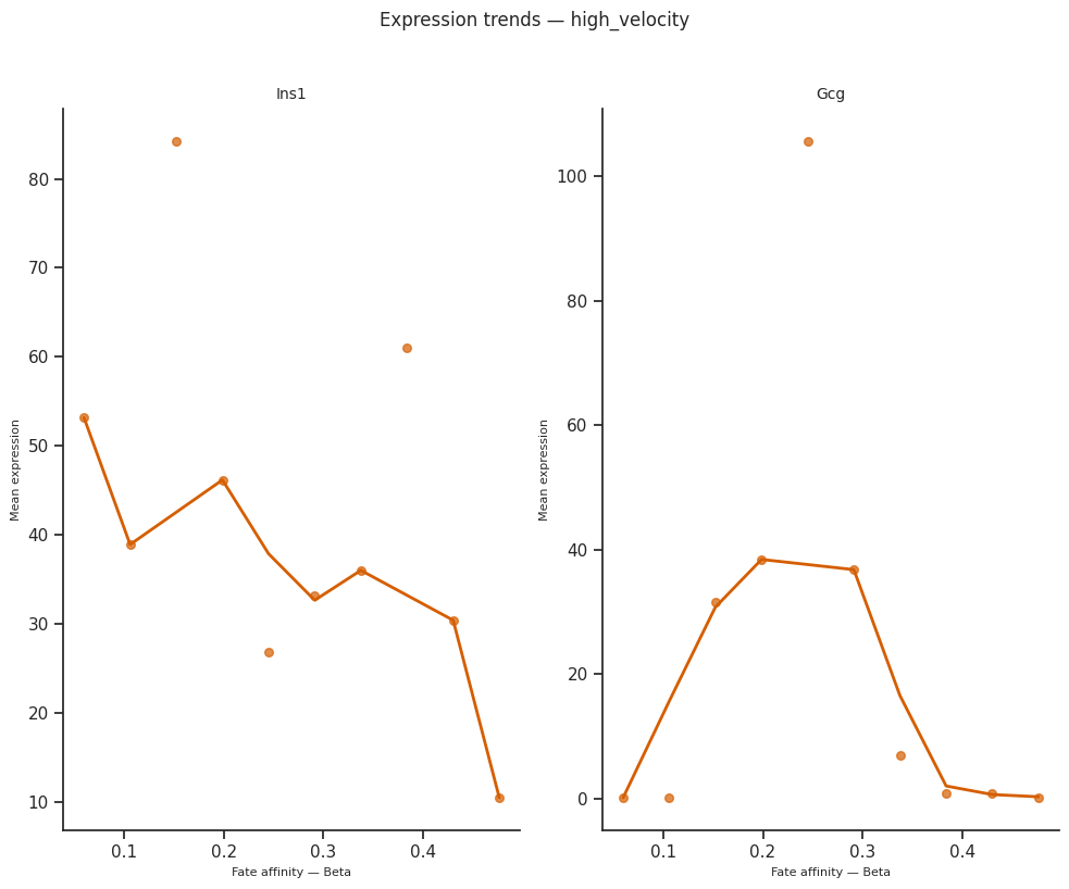
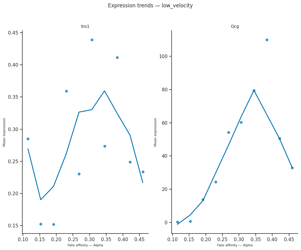
8. Expression trends along fate arms — per condition¶
plot_expression_trends orders cells by per-cell fate affinity (or pseudotime / radial distance) and plots smoothed expression of each gene.
Run it per condition side by side to see whether a marker’s expression trajectory differs between conditions — e.g. earlier onset, higher peak, delayed shutdown.
[31]:
# Expression trends, two markers, side-by-side per condition
from scCS.plot import plot_expression_trends

genes_of_interest = ["Ins1", "Gcg"]  # Beta and Alpha markers
genes_of_interest = [g for g in genes_of_interest if g in adata_sub_shared.var_names]
assert genes_of_interest, "None of the requested markers are in the pancreas var_names"

for cond in mscorer.conditions:
    mask = (adata_sub_shared.obs[mscorer.condition_obs_key].astype(str) == cond).values
    sub = adata_sub_shared[mask].copy()
    try:
        fig = plot_expression_trends(
            sub, results[cond],
            genes=genes_of_interest,
            x_axis="affinity",
            figsize=(10, 4 * len(genes_of_interest)),
        )
        fig.suptitle(f"Expression trends — {cond}", y=1.02, fontsize=12)
        plt.tight_layout()
        plt.show()
    except Exception as e:
        print(f"plot_expression_trends failed for '{cond}': {e}")
9. Transfer labels to full adata¶
transfer_labels() writes per-cell scores from the shared embedding back to the full adata. This is identical to the single-condition workflow.
[32]:
# Transfer per-cell scores to full adata for all conditions
# PairScorer.transfer_labels writes condition-specific columns:
# e.g., cs_high_velocity_Alpha, cs_low_velocity_Alpha, etc.
mscorer.transfer_labels(results, prefix="cs_")

# Columns added to adata.obs
cs_cols = [c for c in adata.obs.columns if c.startswith("cs_")]
print("Columns added to adata.obs:", cs_cols[:8], "...")

# Visualize on UMAP
sc.pl.umap(adata, color=["clusters", "condition"], ncols=2, wspace=0.4)
[scCS] Labels transferred to adata.obs for 1876 / 3696 cells. Columns: ['cs_high_velocity_Alpha', 'cs_high_velocity_Beta', 'cs_high_velocity_Delta', 'cs_high_velocity_Epsilon', 'cs_high_velocity_dominant_fate', 'cs_high_velocity_entropy']
[scCS] Labels transferred to adata.obs for 1876 / 3696 cells. Columns: ['cs_low_velocity_Alpha', 'cs_low_velocity_Beta', 'cs_low_velocity_Delta', 'cs_low_velocity_Epsilon', 'cs_low_velocity_dominant_fate', 'cs_low_velocity_entropy']
Columns added to adata.obs: ['cs_high_velocity_Alpha', 'cs_high_velocity_Beta', 'cs_high_velocity_Delta', 'cs_high_velocity_Epsilon', 'cs_high_velocity_dominant_fate', 'cs_high_velocity_entropy', 'cs_high_velocity_nn_entropy', 'cs_low_velocity_Alpha'] ...
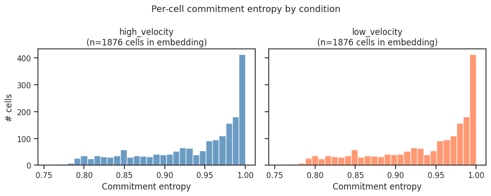
[33]:
# Compare entropy distributions between conditions
# After transfer_labels, columns are named cs_{condition}_{fate}
# For entropy, use the per-condition results directly from adata_sub

fig, axes = plt.subplots(1, 2, figsize=(10, 4), sharey=True)
colors = {"high_velocity": "steelblue", "low_velocity": "coral"}

for ax, cond in zip(axes, ["high_velocity", "low_velocity"]):
    # Get entropy from the condition-specific result
    res = results[cond]
    if res.cell_scores is not None:
        # Compute per-cell entropy from cell_scores
        k = res.cell_scores.shape[1]
        with np.errstate(divide="ignore", invalid="ignore"):
            log_s = np.where(res.cell_scores > 0, np.log(res.cell_scores), 0.0)
        ent = -np.sum(res.cell_scores * log_s, axis=1) / np.log(k)
        ax.hist(ent, bins=30, color=colors[cond], edgecolor="white", alpha=0.8)
        ax.set_title(f"{cond}\n(n={len(ent)} cells in embedding)")
        ax.set_xlabel("Commitment entropy")
        print(f"{cond}: mean entropy = {ent.mean():.3f} ± {ent.std():.3f}")
    else:
        ax.set_title(f"{cond}\n(no cell-level scores)")

axes[0].set_ylabel("# cells")
plt.suptitle("Per-cell commitment entropy by condition", fontsize=13)
plt.tight_layout()
plt.show()
high_velocity: mean entropy = 0.936 ± 0.063
low_velocity: mean entropy = 0.936 ± 0.063
Summary — scCS pairwise workflow¶
import scCS

# 1. Add condition column to adata.obs (or use existing one)
adata.obs["condition"] = ...   # e.g., 'control', 'treated'
adata.obs["sample"] = ...      # biological replicates

# 2. Initialize PairScorer
mscorer = scCS.PairScorer(
    adata,
    root="Ductal",
    branches=["Alpha", "Beta", "Delta", "Epsilon"],
    condition_obs_key="condition",
    obs_key="clusters",
)

# 3. Build SHARED embedding on pooled data
mscorer.build_embedding(ordering_metric="pseudotime")
mscorer.refit_pseudotime(scale_01=False)  # preserve ordering
mscorer.fit()

# ── Tier 1: Score each condition ──────────────────────────────────────────────
results = mscorer.score_all_conditions(cell_level=True, n_bootstrap=200)
mscorer.plot_star_grid(results)
mscorer.plot_rose_grid(results)                    # per-condition rose plots

# ── Tier 2: Statistical comparison ───────────────────────────────────────────
delta = mscorer.compute_delta_CS("treated", "control", n_bootstrap=500)
stats = mscorer.compare_conditions(results, n_permutations=1000)
mscorer.plot_affinity_distributions(results, plot_type="violin")

# ── Tier 3: Trajectory-level analysis ────────────────────────────────────────
lmm   = mscorer.fit_mixed_model(results, replicate_key="sample")
shift = mscorer.trajectory_shift(results, n_bootstrap=500)
mscorer.plot_trajectory_shift(shift)

# ── Downstream §6: Driver genes per condition ────────────────────────────────
# Loop conditions: mask adata_sub per condition, call get_velocity_drivers /
# get_deg_drivers, then collect into one (condition, fate, gene) table.

# ── Downstream §7: Pathway enrichment per condition ──────────────────────────
# Loop conditions: call run_enrichment_per_fate on the per-condition DEG
# drivers, collect into one (condition, fate, direction, Term) table.

# ── Downstream §8: Expression trends per condition ───────────────────────────
# Loop conditions: call plot_expression_trends on the masked adata_sub plus
# results[cond] for side-by-side per-condition trajectories.

# ── Transfer per-cell labels back to full adata for UMAP / downstream ────────
mscorer.transfer_labels(adata, results)
Interpretation guide¶
Result |
Interpretation |
|---|---|
ΔnCS > 0, CI excludes 0 |
Condition A has stronger commitment toward that fate pair |
Permutation p < 0.05 |
Per-cell fate affinities differ significantly between conditions |
LMM condition coefficient significant |
Condition effect on fate affinity, controlling for replicate |
KS p < 0.05 + large Wasserstein |
Cells in one condition are systematically further along the trajectory |
Top driver gene present in one condition only |
Condition-specific regulator candidate |
Pathway enriched in one condition only |
Differentially activated pathway |
Expression trend earlier/later in one condition |
Shifted developmental timing for that gene |
For single-condition analysis, see Single Condition Analysis.ipynb. For 3+ condition analysis, see Multiple Comparison Analysis.ipynb.